Introduction

Decentralized lending protocols rely on effective interest rate models (IRMs) to balance capital efficiency and risk management, and which are adaptable to evolving market conditions. IRMs directly determine the cost of borrowing and the incentives for supplying liquidity and are therefore central to a functioning lending market.

The subject of this report focuses on Curve's Llamalend markets, which have been observed to require additional research and continuous monitoring for performance optimizations. We have seen in the past that LlamaLend markets have experienced low utilization, which degrades returns to lenders and is not an efficient use of capital. More recently, markets have suffered from high utilization, [2], which can prevent lenders from withdrawing and potentially erodes trust in the lending market.

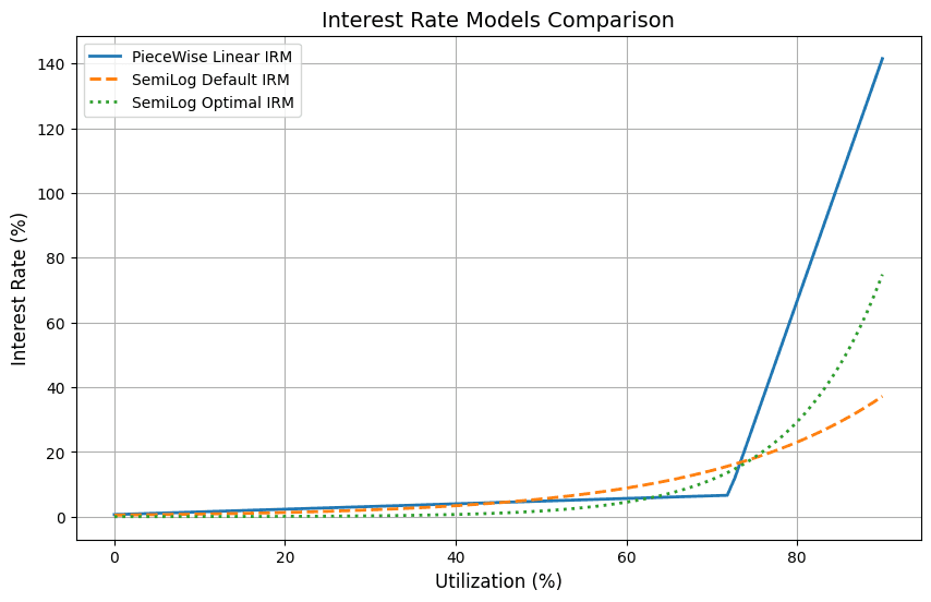
This research addresses the challenge of parameterizing and optimizing IRMs by formally defining the concept of optimal utilization and introducing a framework to optimize and compare different IRM models. As part of the analysis, we review several existing Semilog IRM LlamaLend markets and benchmark their performance against Piecewise Linear IRMs, which are widely used by protocols like Aave and Compound.

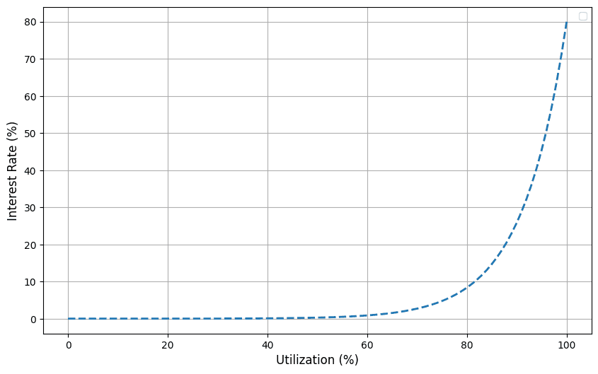
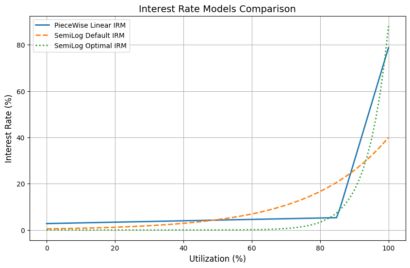
Semilog IRM:

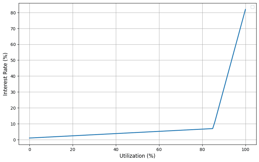
Piecewise Linear IRM:

To summarize, the objectives of this project are three-fold:

1. Define and identify a concept of Optimal Utilization

2. Parameterize the existing Semilog IRM optimally

3. Compare optimality between different IRMs

Section 1: Methodology

We break down the methodology into two distinct parts:

1. Identifying Optimal Utilization

2. Optimization and exploration of IRMs.

1.1 Identifying Optimal Utilization

1.1.1 Background: Conceptualizing Optimal Utilization

To define optimal utilization:

in a lending market, we must balance the needs of borrowers, suppliers, and the protocol itself. As Goldmann et al. (2023) explain, the core challenge lies in determining a utilization level that maximizes collective welfare while minimizing conflicts between stakeholders. Borrowers prefer lower borrowing rates, suppliers seek higher returns, and the protocol benefits from minimizing the spread between these rates.

At first glance, maximizing utilization might seem ideal, as it enhances capital efficiency. However, full utilization (i.e. 100%) creates a critical issue for suppliers. When all liquidity is utilized, suppliers cannot withdraw their funds, degrading user experience and increasing risk for suppliers.

Therefore, optimal utilization is not simply about maximizing efficiency but identifying the highest safe utilization level where the protocol remains operational and withdrawals are feasible. The portion of supply not utilized serves as risk capital, safeguarding the protocol against liquidity and operational risks.

Note: In pool-based lending protocols, full utilization also introduces liquidation risks. When liquidators cannot access underlying tokens to cover underwater positions (relying instead on illiquid representations, such as aTokens), they face inventory risks until utilization drops, potentially jeopardizing the protocol's solvency.

1.1.2 Identifying Optimal Utilization in LlamaLend Markets

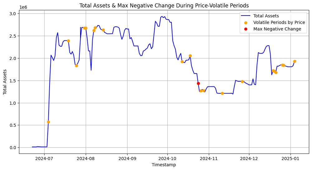
To determine the optimal utilization in LlamaLend Markets we take a supplier-centric view, as Borrowers already benefit significantly from the soft liquidations mechanism. In practical terms, we want to ensure that suppliers can reliably withdraw their funds, even during periods of increased market stress.

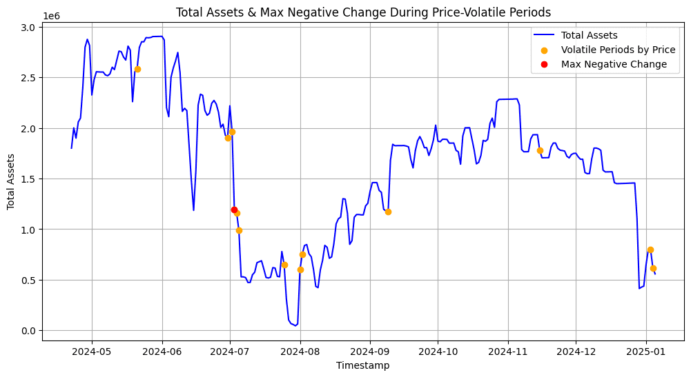
To define:

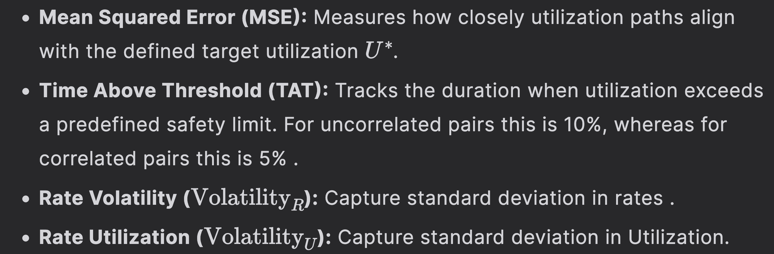
we analyze supplier withdrawal behavior during volatile market conditions. Volatile periods are identified by analyzing price oracle data, where daily price changes exceed a defined threshold to signal significant market fluctuations. Currently, we establish the threshold as 2x the standard deviation of historical changes for uncorrelated collateral-borrow pairs and 1.5x the standard deviation of historical changes for correlated collateral-borrow pairs. We identify the 10th percentile of withdrawals of supplied assets during these periods. This means that 90% of all observed values during volatile periods were less than or equal to this percentage.

Optimal utilization is then derived using a minimum withdrawal buffer, ensuring that sufficient liquidity remains idle to meet peak potential withdrawal demands. Here, optimal utilization is calculated as:

where W represents the highest observed withdrawal activity as a percentage of the total supplied liquidity at the time. For instance, if peak withdrawals at the 90th percentile amount to 25% of the supplied asset, the protocol can safely operate at up to 75% utilization.

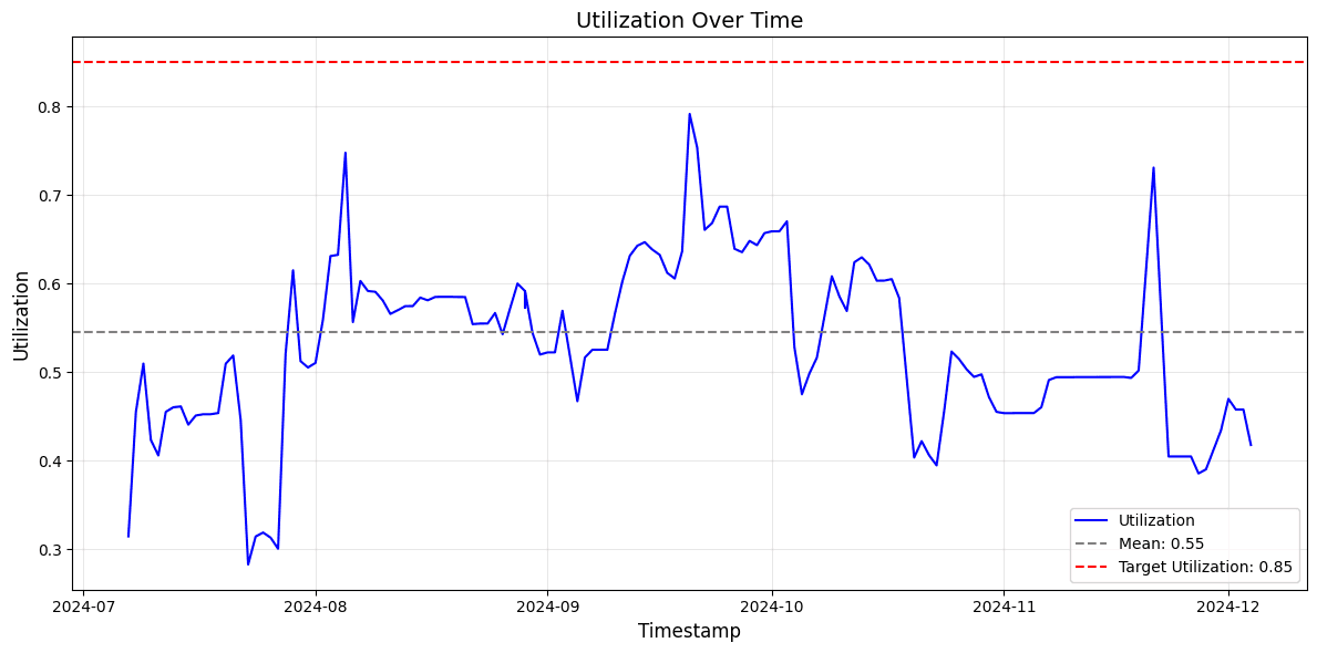
In order to leave sufficient room for growth of the market, we set a growth buffer to 15%. Should the peak withdrawals at the 90th percentile amount to less than 15%, the optimal utilization is set to 85%, as in:

Note: How utilization optimality is defined is something that can be adjusted and largely depends on the priorities of the Curve Community. For instance, less conservative measures could be chosen (i.e. the average of withdrawals during volatile periods, 75th percentile) or entirely different utilization models incorporating additional stakeholders could be considered.

1.2 A General Framework for Parameterizing and Comparing IRMs

To effectively manage utilization rates around optimal utilization, we employ a stochastic modeling framework where we directly simulate synthetic utilization paths. We are able to avoid directly studying and simulating borrow and supply behavior, as utilization is a function of borrow and supply dynamics, and hence, we are able to implicitly capture user behavior purely through the utilization rate. Further reading on this simplified approach can be found in Bertucci et al. (2024).

1.2.1 A Simple Model of Utilization

The model dynamics can be described by:

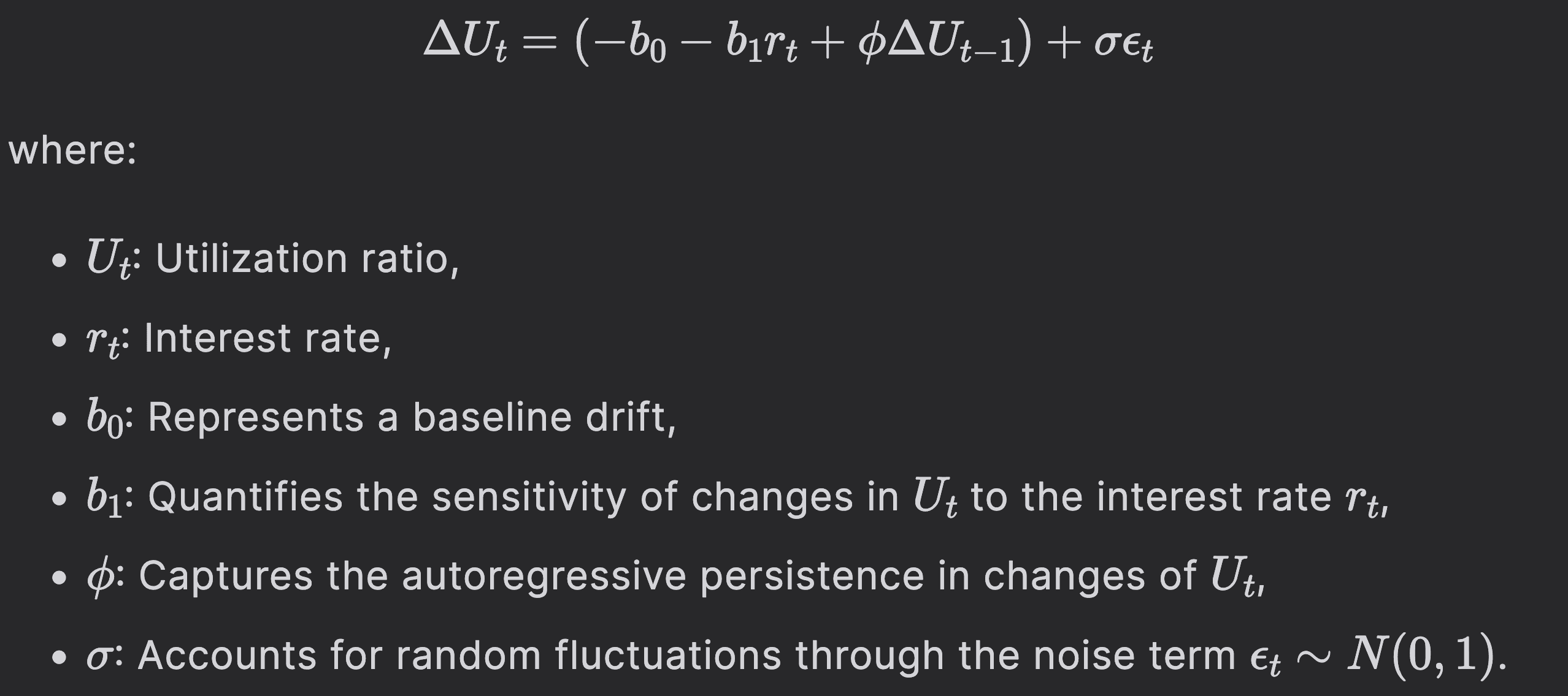
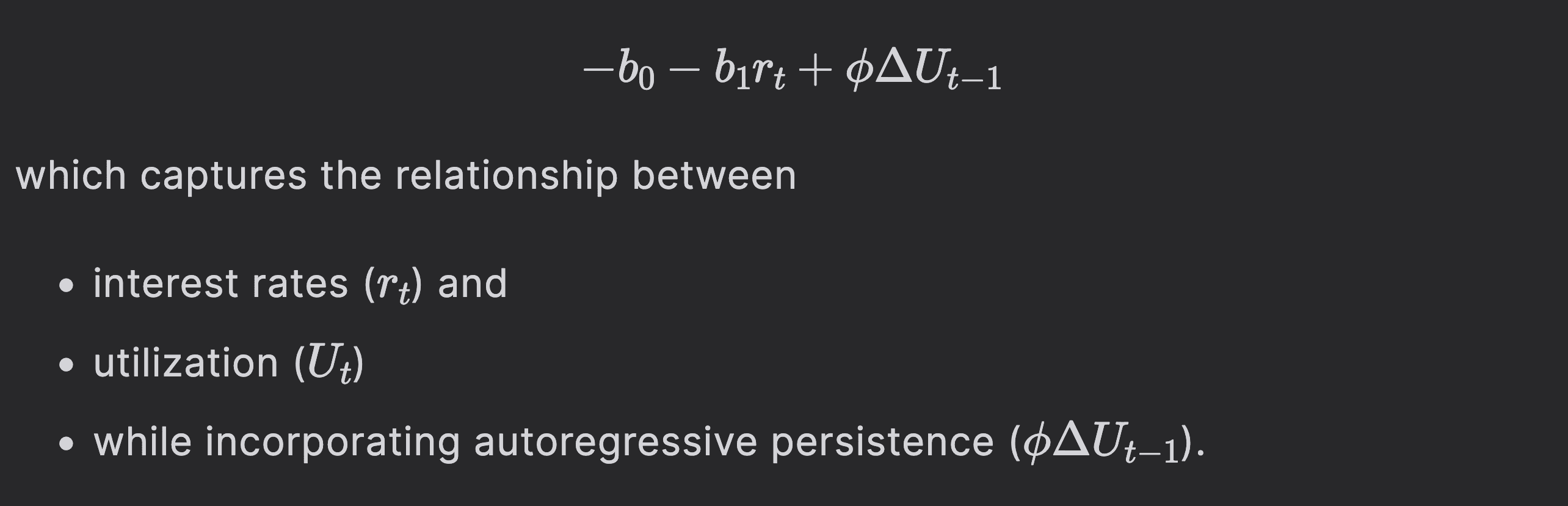
The deterministic term:

models the natural adjustment in utilization driven by interest rate effects and the persistence of past utilization changes, while the stochastic term introduces market noise.

1.2.2 Parameterization of Model Dynamics

To parameterize the model, we utilize daily averages for:

retrieved from the Curve Prices API. In decentralized lending, interest rates depend on the utilization ratio, while the utilization ratio also changes in response to the borrow rate. This feedback loop makes it hard to determine whether borrow drives changes in utilization, or vice versa. In order to address reverse causality, lagged interest rates:

are used, ensuring the model captures the effect of past borrow rates on future delta utilization ratios, avoiding mutual dependence.

The autoregressive term:

is particularly important as it captures the persistence in utilization changes. For example, if utilization has recently increased or decreased, this trend often carries forward to subsequent periods due to market inertia or delayed borrower responses. Including this term ensures the model realistically reflects how past utilization changes influence current dynamics.

We can estimate this using a simple Ordinary Least Squares (OLS) regression of the form:

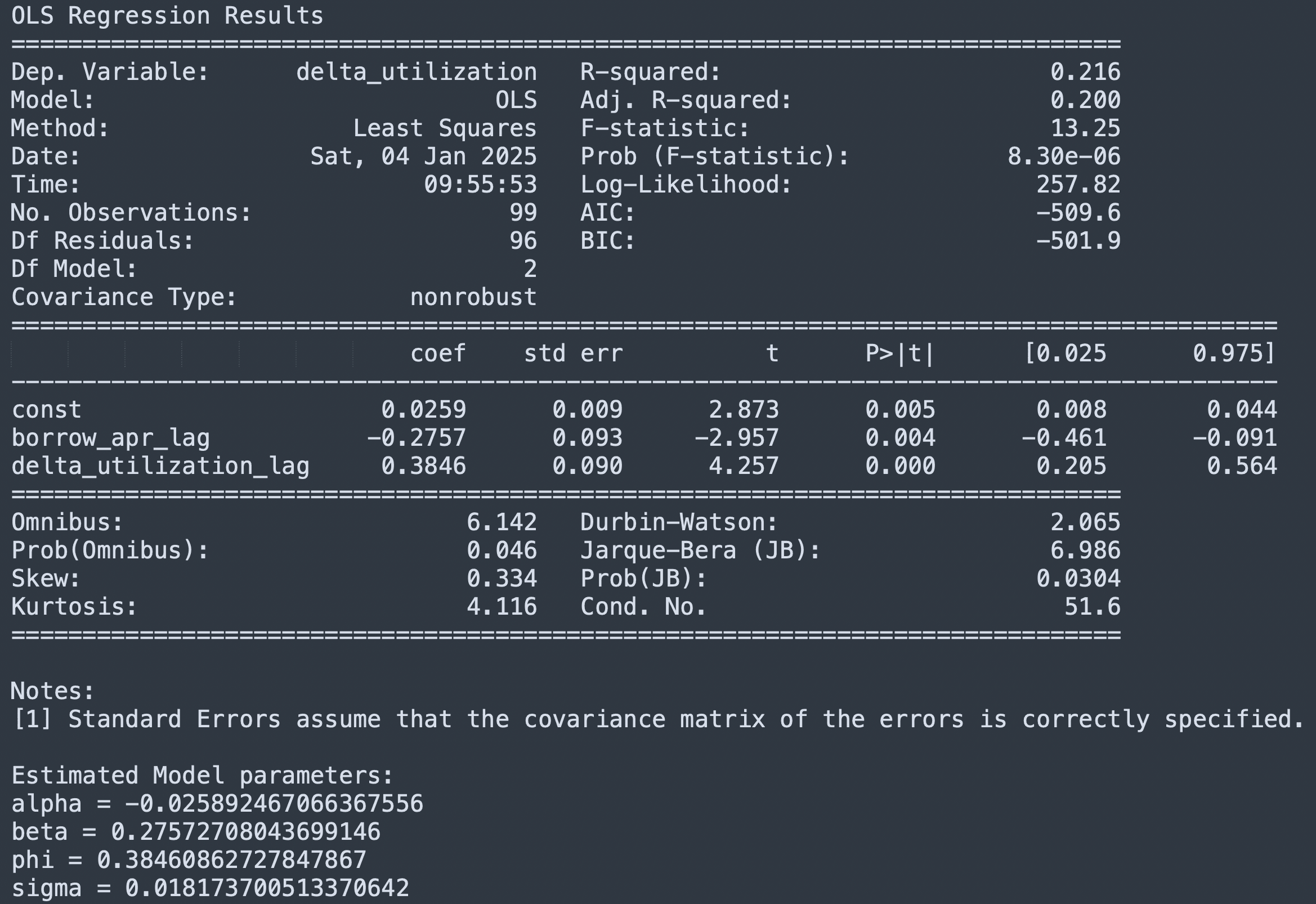
While explanatory power (R-squared) is often low, we find that a statistically significant relationship between interest rates and utilization confirms a meaningful, consistent effect. Given our objective is not for prediction but for studying core dynamics, it makes it useful for optimizing IRMs and guiding utilization calibration. Sigma is parameterized using the residual Mean Square Error (MSE) of the OLS regression.

1.2.3 Modeling Assumptions

The model assumes a linear drift term:

This term accounts for both the direct impact of interest rates and the continuation of past trends, providing a more dynamic representation of utilization changes.

The diffusion term:

assumes constant volatility over time, simplifying the analysis but potentially overlooking heightened market uncertainty during stress periods. This assumption makes the model particularly suitable for stable market conditions but may require adjustments when applied to volatile or crisis scenarios. In practical terms, as we optimize the market for equilibrium dynamics this makes this model suitable for this.

By focusing on stationary dynamics through lagged inputs like:

the model avoids distortions from long-term market growth or structural changes. This approach ensures that short-term behaviors are isolated and well-represented, making the model useful for optimizing IRMs under stable conditions. However, in evolving or rapidly changing markets, reparameterization of the model will be necessary to maintain its accuracy and relevance.

1.2.4 Simulation of Interest Rate Models

We evaluate the performance of different interest rate models by simulating utilization and interest rates. For each simulated path, key performance metrics are calculated to assess model efficiency and stability. The following metrics are captured:

1.2.5 Optimization Settings

To fine-tune parameters, we employed the CMA-ES (Covariance Matrix Adaptation Evolution Strategy) optimizer. The optimization process targeted the minimization of the weighted loss function. The proceeding analysis introduced a composite loss function with weights:

• MSE = 10,

• TAT = 0.01,

• Volatility_R = 1.0

For the optimizer, we introduce an inverse metric to TAT with a "Time Below Threshold". This is given a minor weight of 0.001 to counter under-utilization.

We are able to adjust weights and feed arbitrarily weighted composite loss functions to the optimizer which allows prioritization of specific objectives (e.g., 2x MSE, 1x Volatility_R). This provides flexibility in tailoring the optimization to address varying performance requirements or preferences of the Curve Community (e.g. rate stability vs close tracking of optimal utilization).

We tuned the hyperparameter for the CMA-ES Optimizer based on the best score of the objective function, accounting for variation across paths and the parameter set that generally leads to stability in optimal parameters across restarts. Due to time constraints, we went with one generalized setting across all markets for the Semilog policy and Piecewise Linear function, respectively. We tested the parameter difference for maximum iterations until convergence, the number of paths, and sigma. We kept:

• popsize = 8,

• restarts = 2,

• incpopsize = 1.2 and

• tolx = 1e-6

In order to avoid overfitting, we varied the initial guess by between 75% to 150% of the current default parameters. In addition, the input data varies by default as the utilized stochastic elements in the utilization paths.

In order to avoid capturing periods where the model might not have settled into an equilibrium state, we take the second half of the simulated paths to capture the evaluation metrics.

• Optimization steps: 30 iterations

• Simulation paths: 100

• Optimizer Sigma: 1.0

Section 2: Results

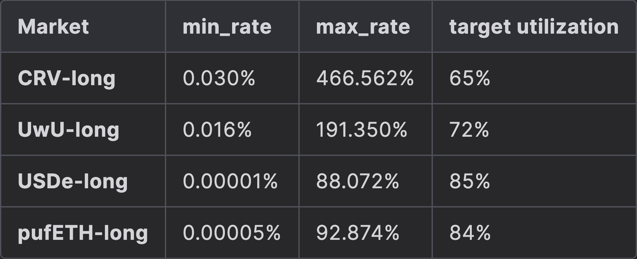
We applied our methodology to 4 Semilog LlamaLend markets: CRV-long, UwU-long, USDe-long, and pufETH-long, and compared the default parameters to the optimized parameters and to a Piecewise Linear IRM Model.

A summary of Semilog optimization results (the existing IRM for the target markets) is given in the table below:

2.1 LlamaLend Market: CRV-long

The CRV-long Market was deployed on 2024-03-14 with the current interest rate parameters min_rate = 1.0% and max_rate = 80.0%.

2.1.1 Identifying U_optimal

We identify volatile periods (i.e. 2x the daily standard deviation) based on the price oracle feed and then identify the 10th percentile of withdrawals of supplied assets during these periods.

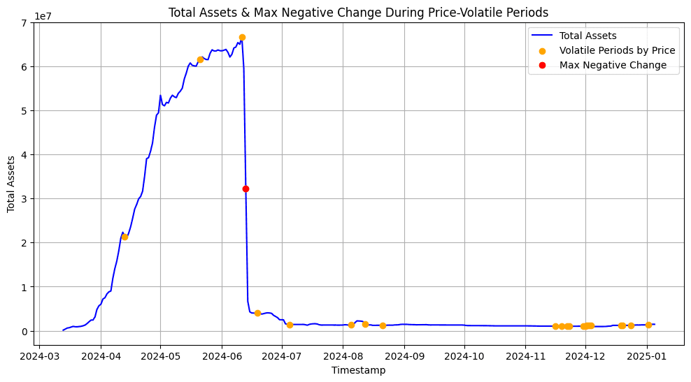
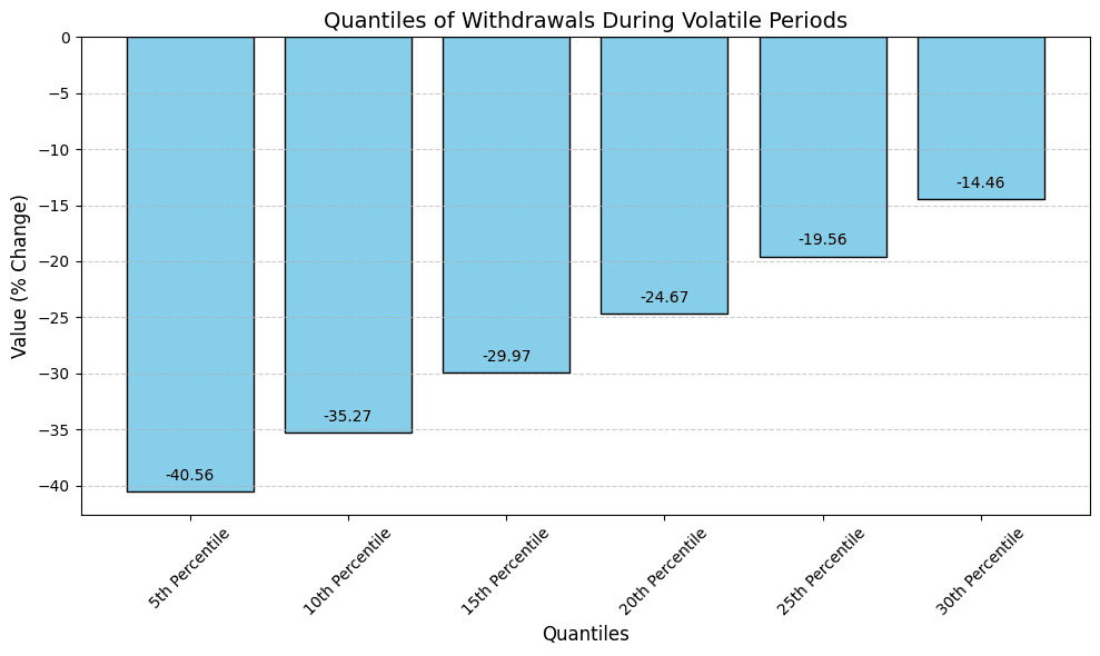
The 10th percentile of negative withdrawals of supplied crvUSD during volatile periods was -35.27% of the total supply. This means that 90% of all observed withdrawals during volatile periods were less than or equal to this value. Based on this, we define the optimal utilization rate as 65% (65% = 100% - 35%).

2.1.2 Studying IRM Models

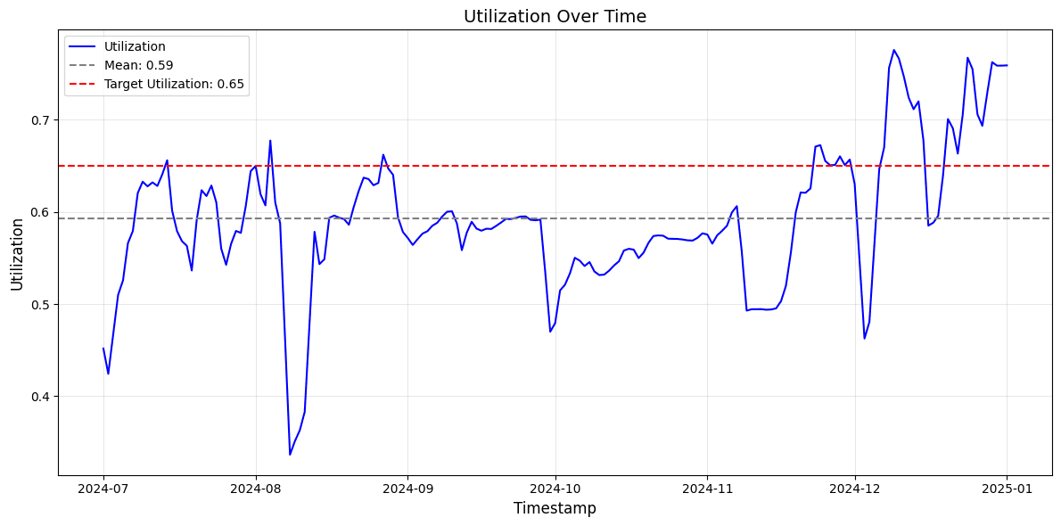
We select the last 6 months of data for this market and parameterize our model to it.

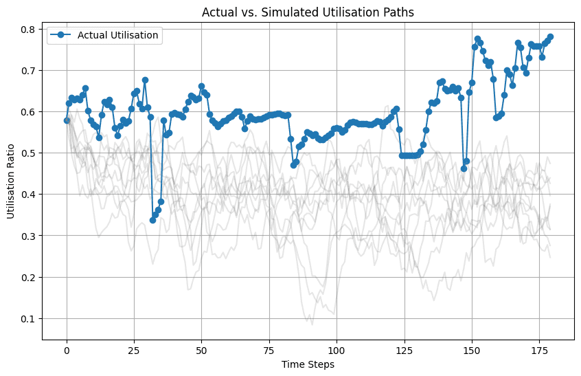
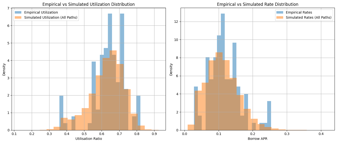
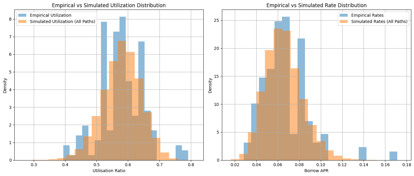
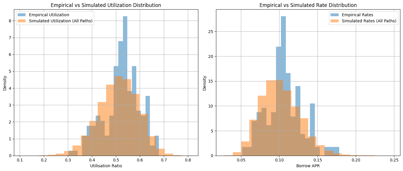
We see that the average utilization of the market, according to our methodology, is underutilized. The mean utilization in the observation period (59%) is lower than the target rate of 65%.

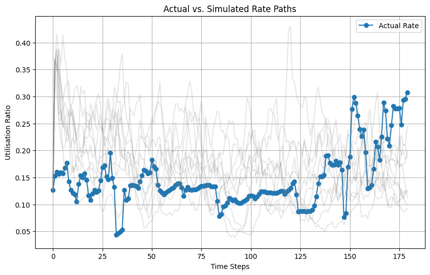
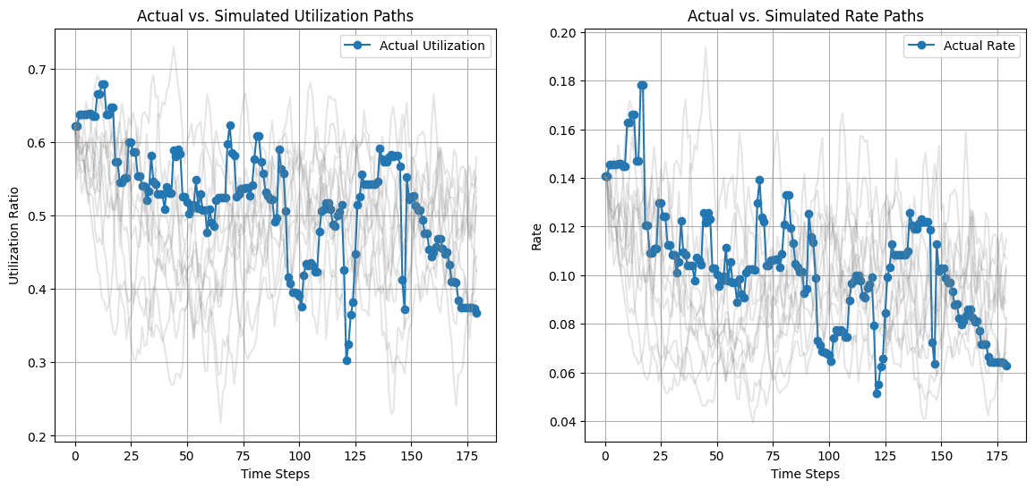
To sanity-check the model, we run the simulation with the default IRM parameters to see if we are able to replicate the empirical distribution of the sample period reasonably well. While skew and kurtosis differ somewhat, overall the replicated distribution of utilization and rate is replicated well with our model and produces realistic paths.

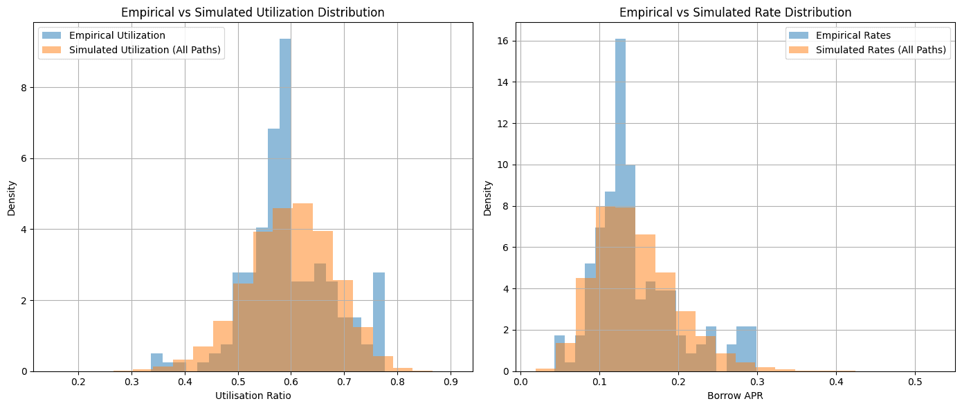
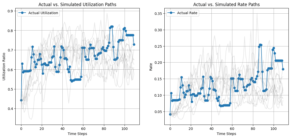
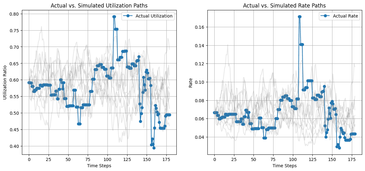
The charts below show the utilization and rate paths of the actual market (blue) against the simulated paths (gray).  

2.1.3 Optimization of IRM Parameters

The optimization process purely focuses on minimizing the composite loss function and leads to the following parameters for each interest rate model:

• SemiLog IRM: The optimal parameters for the semilog model in the current market regime are rate_min= 0.03% and rate_max=466.562%.

• PieceWiseLinearIRM Optimization: The optimal parameters for the semilog model in the current market regime are r0=0.002, r1=0.148, r2=9.214.

2.1.4 Comparison of IRM Models Across Key Metrics

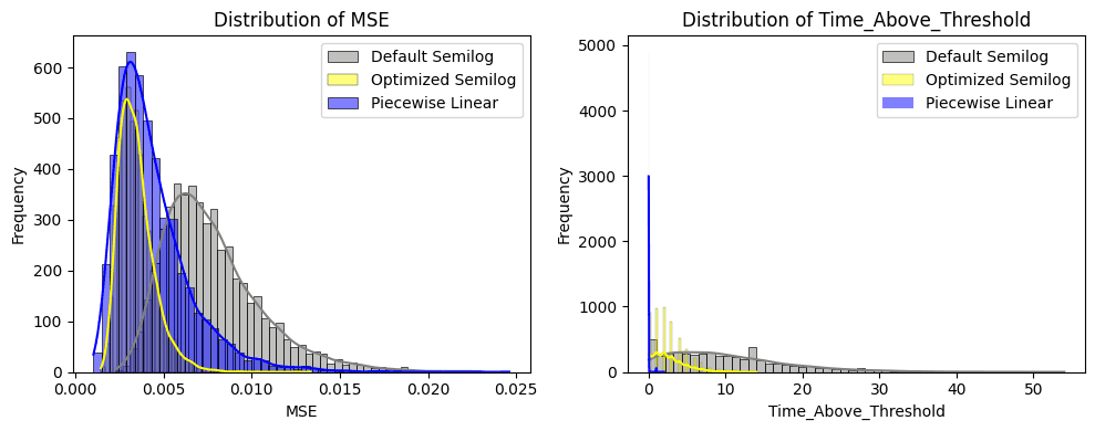
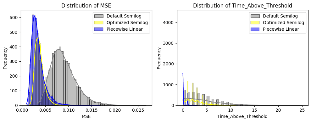
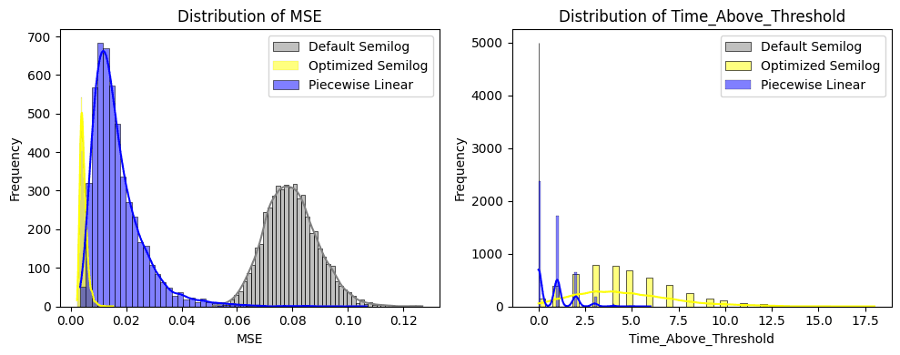
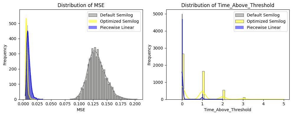
On the left chart (below), we see the Mean Square Error (MSE) from the optimal utilization in absolute terms across 5000 validated paths with the parameter configuration of the respective IRM. We see that the Optimized Semilog Model (yellow) performed best with a narrow spread and the lowest mean. The Piecewise Linear Model performed second best with a slightly higher mean but much larger spread, suggesting it is less successful to manage utilization around the Optimal Utilization level.

On the right chart (below) we see the distribution of the Time Above Threshold (TAT) metric. The metric gets triggered if the market deviates more than 10% from the target utilization. The Piecewise Linear Function (blue) manages to best avoid over-utilization. Yet, viewing it in combination with the MSE suggests that it overcorrects, leading to a large deviation under the target utilization due to aggressive rate increases when the optimal utilization level is overshot. The optimized Semilog IRM (yellow) experiences some persistent levels over target utilization but performs better than the default configuration of the Semilog model (grey).

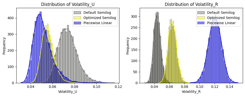
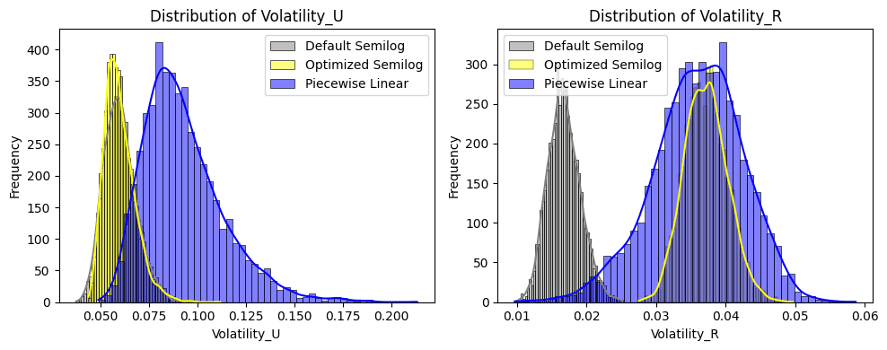
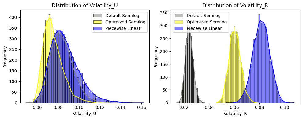
The distribution of utilization rate volatility is shown in the left chart below. We see that the Piecewise Linear (Blue) manages to minimize the volatility in the utilization, followed by the Optimized Semilog policy. The worst configuration is from the default configuration.

The distribution of borrow rate volatility is displayed in the right chart, showing the rate volatility across the simulated paths. It is apparent that the default configuration shows the lowest rate volatility, followed by the optimized Semilog and finally by the Piecewise Linear IRM.

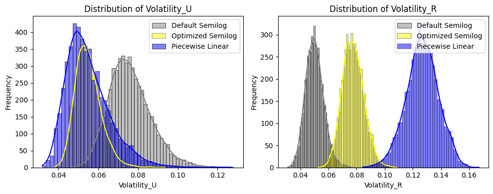
The results charts highlight that the optimized policies achieve superior performance in MSE and TAT by increasing their sensitivity to rate changes. This leads to more volatility, as over-utilization is more heavily penalized with higher rates. This defines the natural trade-offs that policy configurations attempt to balance.

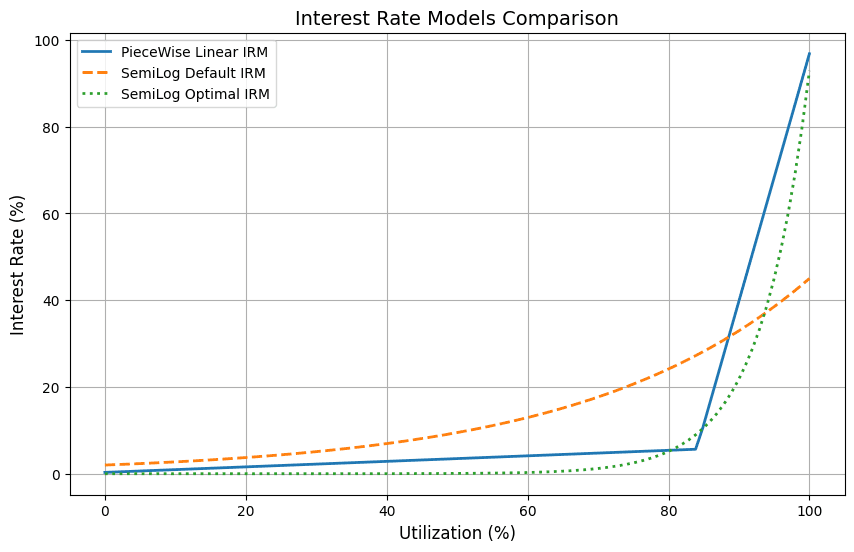
2.1.5 Comparing the Policy Functions

The Optimized Semilog Model suggests substantially lower rates than the default configuration when below the target utilization, while aggressively raising rates above a utilization of around 67%. In practical terms, it heavily incentivizes borrowing at low rates. Further investigation is warranted to determine whether suppliers can be sufficiently incentivized.

The Piecewise Linear model is more generous to suppliers but favors borrowers more around the target. It heavily punishes utilizations above the target utilization.

Both optimized Semilog and Linear Piecewise try to offer lower rates. This makes sense given that the empirical mean of the current market is 59% over the study period, while the target utilization is set at 65%, thus encouraging cheaper borrowing rates at the target to increase utilization. A change in IRM parameters or model is advisable in this market if stakeholders value more stringent protection of the optimal utilization level.

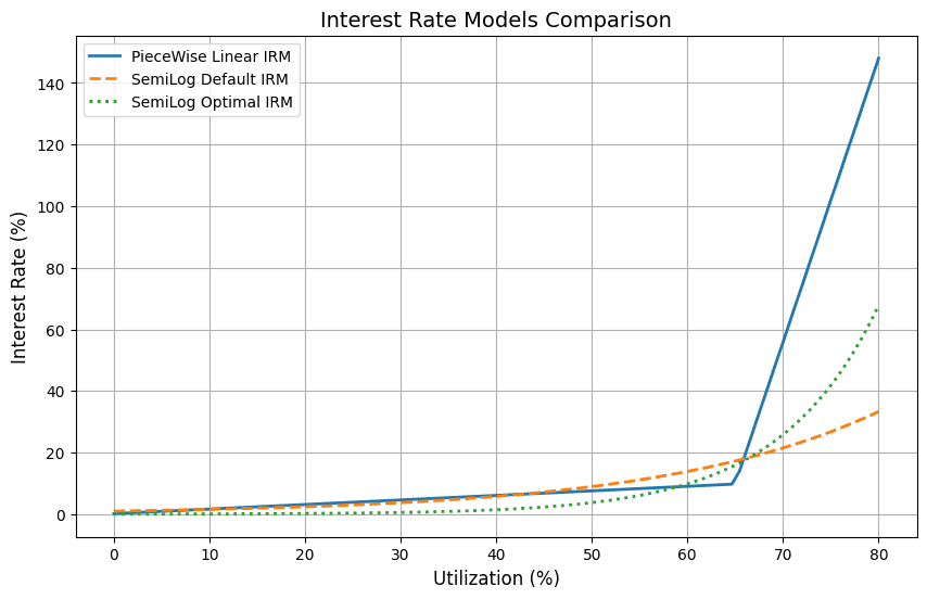
*Note: We cropped the Utilization Rate to 80% to be able to more closely study the dynamics at the target utilization level.*

2.2 LlamaLend Market: UwU-long

The UwU-long market was deployed on 2024-04-22 with the default parameters min_rate = 0.5% and max_rate = 60.0%.

2.2.1 Identifying U_optimal

We identify volatile periods (i.e. 2x the daily standard deviation) based on the oracle price feed and then identify the 10th percentile of withdrawals of supplied assets during these periods.

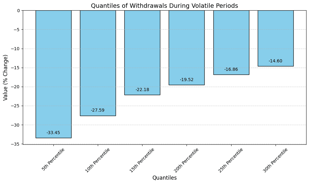
The 10th percentile of negative withdrawals of supplied crvUSD during volatile periods was -27.59% of the total supply. This means that 90% of all observed withdrawals during volatile periods were less than or equal to this value. Based on this, we define the optimal utilization rate as 72% (i.e. ~ 100% -28%)

2.2.2 Studying IRM Models

We select the last 3 months of data (as the stationary assumption in our model is violated and the market appeared to undergo a material change).

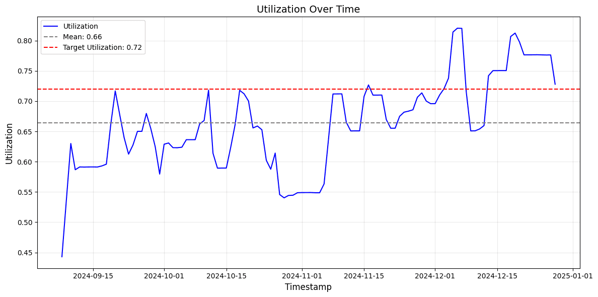
As visible in the figure above, the market is underutilized according to our methodology. The target utilization is 72% compared to the current mean of 66%.

We sanity-check the model by running the simulation with the default IRM parameters to see if we are able to replicate the empirical distribution of the sample period reasonably well.

The charts below demonstrate the market's actual utilization and rate paths (blue) against the simulated paths (gray).

2.2.3 Optimization of IRM Parameters

The optimization process, when purely focusing on minimizing the MSE, leads to the following parameters for each interest rate model:

• SemiLog IRM: The optimal parameters for the Semilog model in the current market regime are rate_min= 0.016% and rate_max=191.35%.

• PieceWiseLinearIRM Optimization: The optimal parameters for the semilog model in the current market regime are r0=0.007, r1=0.083, r2=7.495.

2.2.4 Comparison of IRM Models Across Key Metrics

In the left chart (below) we display the distribution of the MSE across 5000 paths for each IRM. The Optimized Semilog IRM (yellow) and Piecewise Linear IRM (Blue) achieve a lower MSE compared to the default configuration, reducing the error to the Target Utilization. The optimized Semilog maintains a lower spread compared to Piecewise Linear.

The right chart (below) shows the days that the utilization spends above the target utilization with a buffer of 10%. Given that the UwU market is underutilized compared to our target rate, the default Semilog IRM (gray) unsurprisingly only spends a few days above the target utilization. The Optimized Semilog Model (yellow) performs worst, with substantial periods spent above the target utilization. Finally, the Piecewise Linear IRM (blue) seems to perform best with the least days spent above the target utilization.

The left chart (below) depicts the distribution of utilization volatility, showing that both the Piecewise Linear and Semilog Model lead to lower levels of utilization rate volatiltiy compared to the default model. Being lower than the default configuration suggests that utilization levels are more stable.

As seen in the CRV-long market, the distribution of the borrow rate volatility (below right chart) highlights that the optimized Semilog and Piecewise Linear achieve superior control through responsiveness in rate, resulting in higher rate volatility.

2.2.5 Comparing the Policy Functions

Both Piecewise Linear and optimized Semilog suggest lower rates than the default Semilog model around the target utilization level. The optimized Semilog rate exceeds the default configuration at around 75% utilization. The Piecewise Linear IRM shows an aggressive increase right after the target utilization. Overall, in this market, a Piecewise Linear Model may be better suited under current market conditions.

*Note: We cropped the chart to 90% utilization to better visualize the dynamics around the target utilization of each IRM.*

2.3 LlamaLend Market: USDe-long

The USDe-long market was deployed on 2024-06-22 with the default min_rate = 0.5% and max_rate = 40.0%.

2.3.1 Identifying U_optimal

We identify volatile periods (i.e. 1.5x the daily standard deviation) based on the oracle price feed and then identify the 10th percentile of withdrawals of supplied assets during these periods.

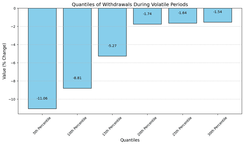
The 10th percentile of negative withdrawals of supplied crvUSD during volatile periods was -8.81% of the total supply. This means that 90% of all observed withdrawals during volatile periods were less than or equal to this value. Based on this, we define the optimal utilization rate as 91% (i.e. ~ 100% - 9%). Yet, given that this threshold is close to full utilization, we apply the growth buffer and set optimal utilization to 85%.

2.3.2 Studying IRM Models

We limited the observation period to 6 months, limiting it to a stable utilization rate period to comply with the stationary assumption of our model.

The market, according to our methodology, is severely underutilized. The observed mean is much lower (55%) than the suggested target utilization level (85%).

To sanity check the model we run the simulation with the default IRM parameters and see if we are able to replicate the empirical distribution of the sample period reasonably well. Both utilization and rate distribution reasonably replicated the empirical distribution.

The historical utilization and rate paths of the actual market (blue) are charted below against the simulated paths (gray).

2.3.3 Optimization of IRM Parameters

The optimization process, when purely focusing on minimizing the objective function, leads to the following parameters for each interest rate model:

• SemiLog IRM: The optimal parameters for the Semilog model in the current market regime are rate_min= 1e-05% and rate_max=88.072%.

• PieceWiseLinearIRM Optimization: The optimal parameters for the PWL model in the current market regime are r0=0.028, r1=0.03, r2=4.896.

2.3.4 Comparison of IRM Models Across Key Metrics

On the left chart (below), we observe the distribution of MSEs. The Optimized policy (yellow) performs best. The Piecewise Linear policy (blue) performs worse under the optimization setting. The default Semilog policy (grey), performs worst with the highest MSE and standard deviation.

The right chart (below) depicts the time above the threshold where utilization remains 5% higher than the optimal utilization. The optimized Semilog spends the longest time above the target utilization, indicating operation in what we consider "unsafe" utilization ratio levels. The Piecewise Linear performs slightly better. The default configuration, due to it under-utilization, performs best by never exceeding the safe threshold.

In the left chart below, we examine the utilization volatility distribution. The Piecewise Linear IRM (blue) demonstrates the most unstable utilization with the highest volatility and spread, followed by the optimized Semilog policy (yellow) and then the Default Semilog (gray).

On the right chart below, we analyze the volatility of the borrow interest rate. Here, the Piecewise policy shows the highest rate volatility and largest standard deviation. Conversely, the Default configuration shows low volatility, which can be explained by the relatively unopinionated shape of the interest rate policy.

2.3.5 Comparing the Policy Functions

Both the optimized Semilog and Piecewise Linear IRM suggest much lower rates compared to the default configuration. Given that the market is underutilized, this is sensible. The Piecewise Linear slope increases very statically until the target utilization, which may indicate adjusted optimization criteria in this market. The optimized Semilog seems more favorable but may be too accommodating to borrowers. Further fine-tuning of the optimization criteria may be needed before updating this market.

2.4 LlamaLend Market: pufETH-long

The pufETH-long market was deployed on 2024-05-05 with the current parameters min_rate = 2.0% and max_rate = 45.0%.

2.4.1 Identifying U_optimal

We identify volatile periods (i.e. 2x the daily standard deviation) based on the oracle price feed and then identify the 10th percentile of withdrawals of supplied assets during these periods.

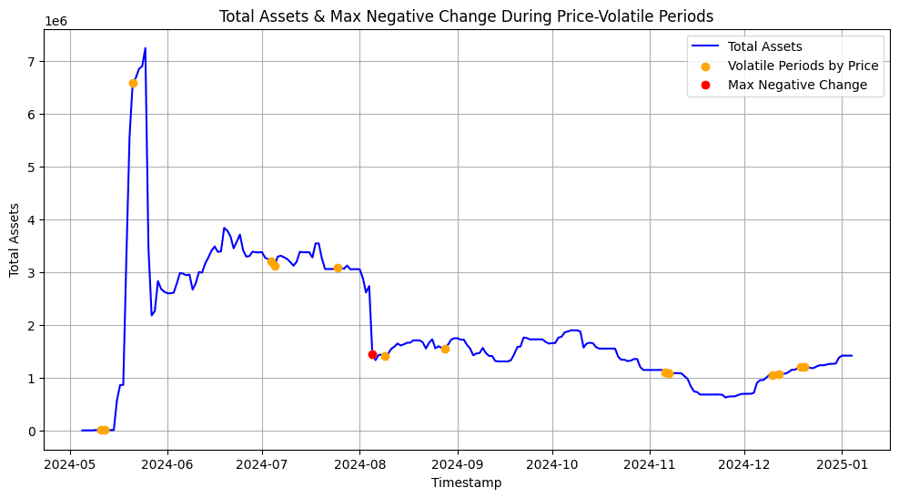
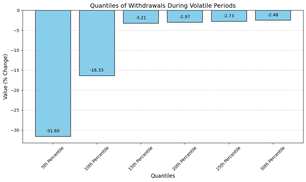
The 10th percentile of negative withdrawals of supplied pufETH during volatile periods was -16.33% of the total supply. This means that 90% of all observed withdrawals during volatile periods were less than or equal to this value. Based on this, we define the optimal utilization rate as 84% (i.e. ~ 100% -16%)

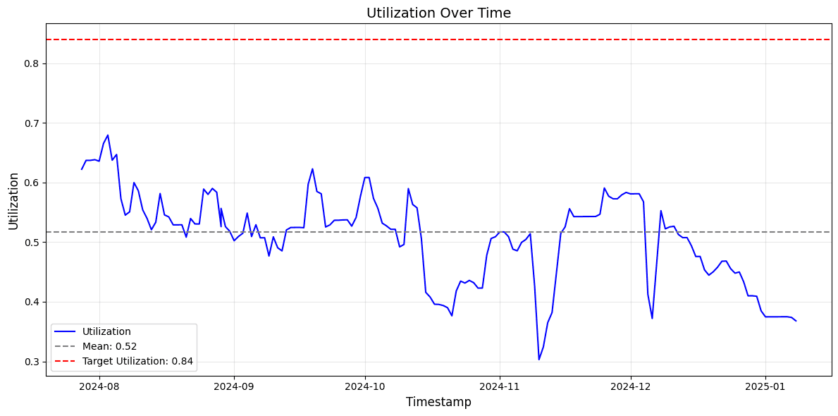
2.4.2 Studying IRM Models

We select the last 6 months of data for this market and parameterize our model to it.

The current market, according to our methodology, is underutilized. The mean utilization during the current period (52%) is below the target utilization of 84%.

In order to sanity check the model, we run the simulation with the default IRM parameters to see if we are able to replicate the empirical distribution of this period reasonably well. The figure below shows that the empirical vs. simulated utilization and rate distribution fit reasonably well.

The chart below shows the utilization and borrow rate paths of the actual market (blue) against the simulated paths (gray).

2.1.3 Optimization of IRM Parameters

The optimization process, when purely focusing on minimizing the MSE, leads to the following parameters for each interest rate model:

• SemiLog IRM: The optimal parameters for the Semilog model in the current market regime are rate_min= 5e-05% and rate_max=92.874%.

• PieceWiseLinearIRM Optimization: The optimal parameters for the PWL model in the current market regime are r0=0.003, r1=0.064, r2=5.697.

2.4.4 Comparison of IRM Models Across Key Metrics

We see in the left chart (below) the MSE distribution of each model. The default Semilog IRM (grey) has the highest MSE compared to target utilization, while the optimized Semilog IRM (yellow) and Piecewise Linear IRM (Blue) perform similarly well.

The right chart (below) shows the Time Above Threshold, where the Default Semilog Model does not appear. The reason for this is that this market has historically been under-utilzied compared to the target utilization level. The optimized Semilog shows up to 5 days above the target utilization with the suggested configurations. The Linear Piecewise model performs best, with a maximum of 2 days above the target utilization.

The left chart (below) shows the distribution of utilization volatility. All models perform similarly, suggesting that utilization levels vary by the same degree.

In the right chart (below) we see the volatility of the rate, which effectively explains how utilization is stabilized. Here, we see inverse behavior. The default Semilog policy generates the lowest variation in rate and Piecewise Linear has the highest overall rate volatility. Both Optimized models achieve this by creating more opinionated curvature around the target utilization compared to the default Semilog model.

2.4.5 Comparing the Policy Functions

The Piecewise Linear and optimized Semilog show much lower rates than the default configuration below the target utilization rate, encouraging borrowing. Rates become more punitive above the target utilization, around 85%-92% utilization.

Conclusion

This research demonstrates a framework for identifying optimal utilization and optimizing interest rate models (IRMs) in decentralized lending protocols. By defining optimal utilization as a balance between capital efficiency and withdrawal feasibility, we ensure market stability while mitigating risks for suppliers. Through stochastic modeling and parameter optimization, we benchmarked the performance of Semilog and Piecewise Linear IRMs across various LlamaLend markets.

The current models shows there is no free lunch - rate stability leads to less responsiveness, potentially leading to more days in "unsafe" utilization levels or deviation from the target utilization, and vice versa. The models studied in this work are limited by their shape in how well they can respond to market dynamics. While the Piecewise Linear at times performed better, it is still far from perfect. Introducing policy-specific weighting schemes during optimization can likely improve parameter suitability. Nevertheless, there is likely a need for the development of more adaptive models.

In addition, the analysis highlights that the current state space defined in the smart contract is too limited for the min_rate in the Semilog MP contracts. Our simulation for USDe-long and pufETH-long recommend parameters currently below the min_rate of 0.1% defined in the smart contract.

In future work, we will explore the Secondary IRM policy, a more adaptive IRM that references an external source to assign an appropriate rate at the target utilization. In addition, there is an opportunity to explore additional IRM models, which we can test and compare to existing models using this framework. The latest literature emphasizes adaptive rate controllers that adaptively set utilization rates on market metrics and explore novel interest curves. We believe that this research can build a foundation for setting more effective IRM policies to build more resilient and efficient LlamaLend markets in the future.

Appendix

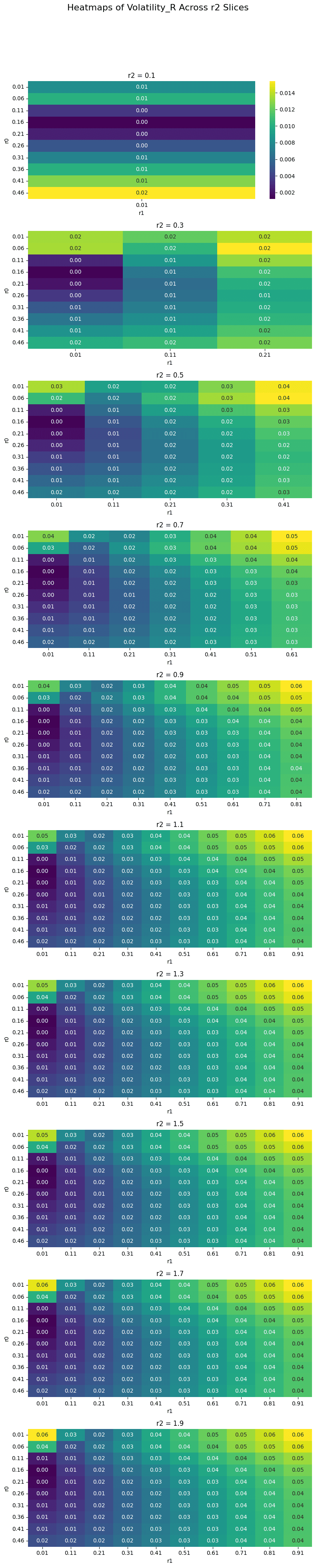
A.1 Sensitivity Analysis

In this section, we show the results of a Sensitivity analysis for the pufETH market on the evaluation metrics. We have the results for the remaining markets and we are happy to share them on request. We excluded them from the report for the sake of brevity.

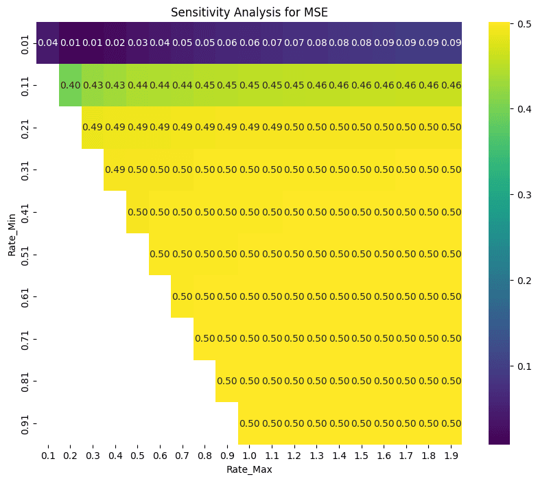
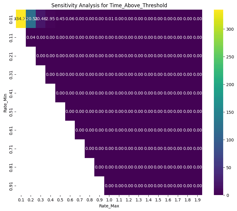
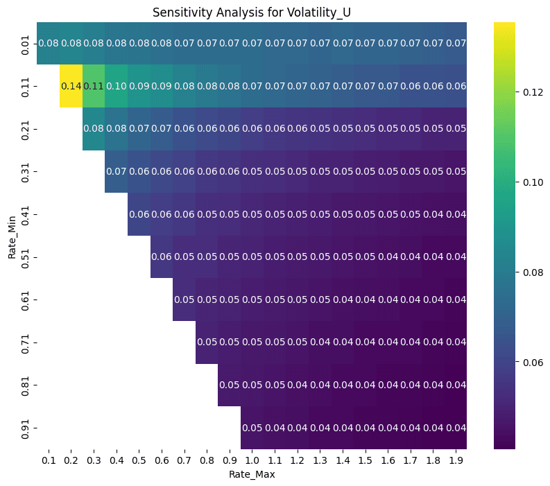
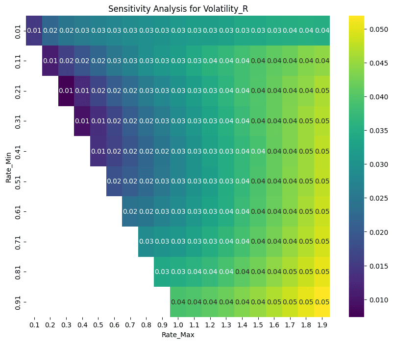
A.1.1 Semilog IRM

The MSE is minimized by choosing a combination of low rate_min and relatively high rate_max. In the case of pufETH, the 200-400% max rate range produces a minimized MSE. This allows the Semilog to most effectively maintain the optimal utilization.

The Time_Above_Threshold is effectively avoided by setting a high max rate. The configuration where this escalates is when choosing a parameter combination where rate_min and rate_max are low. This results in the market consistently being overutilized (i.e. above the target threshold).

The volatility of utilization and rate shows a more interesting pattern. Rate combinations where the difference between rate_min and rate_max are minimized result in low volatility, as the rates effectively become unresponsive to changes in utilization. Diverging combinations exhibit higher volatility as rates become more responsive. Volatility in utilization and rate effectively requires a trade-off with MSE.

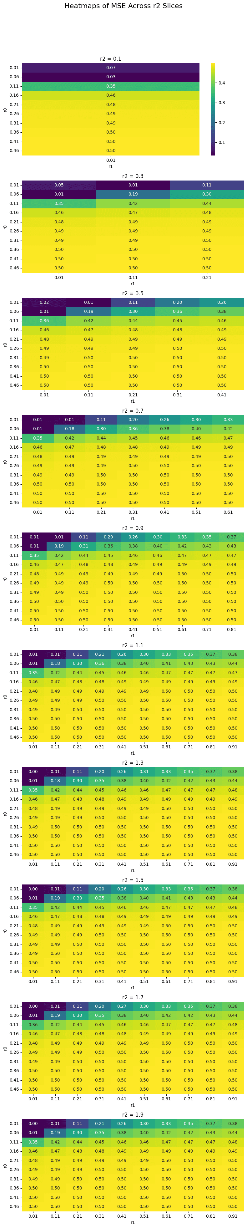
A.1.2 Piecewise Linear IRM

The Piecewise Linear Sensitivity Analysis is slightly more complex, as we study the interactions between 3 parameters (r0, r1, r2). We solve this by slicing and fixing r2.

The MSE seems to be highly influenced by the combination of r0 and r1 in the Piecewise Linear IRM. This makes sense as it effectively manages utilization below optimal utilization. r2 does also play a role in managing MSE. When comparing the absolute values we see that the MSE starts to decrease with a higher r2.

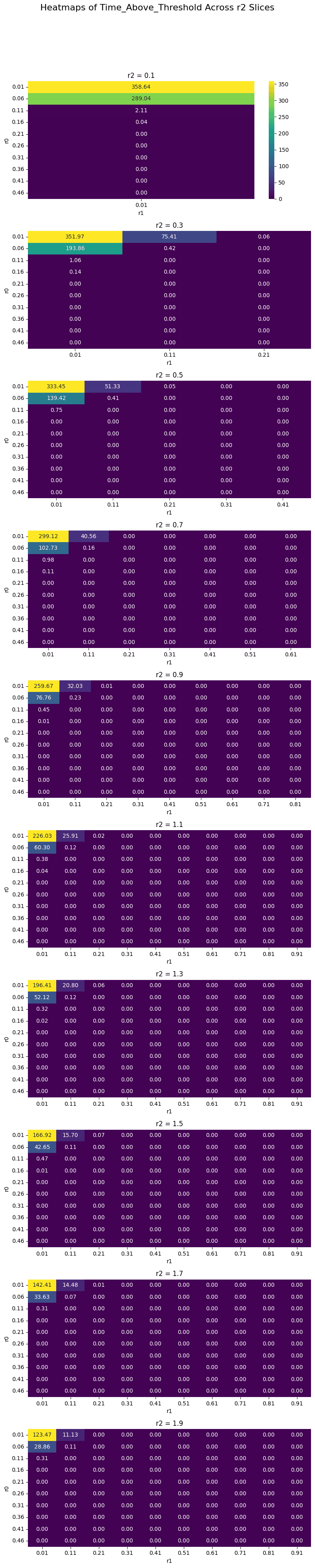
A similar picture is observed when viewing the Time_Above_Threshold, with r2 being largely responsible for controlling the days above threshold.

The volatility of the utilization rate is highly correlated to the divergence between r0 and r1. Again, absolute values tend to decrease with a larger r2 value.

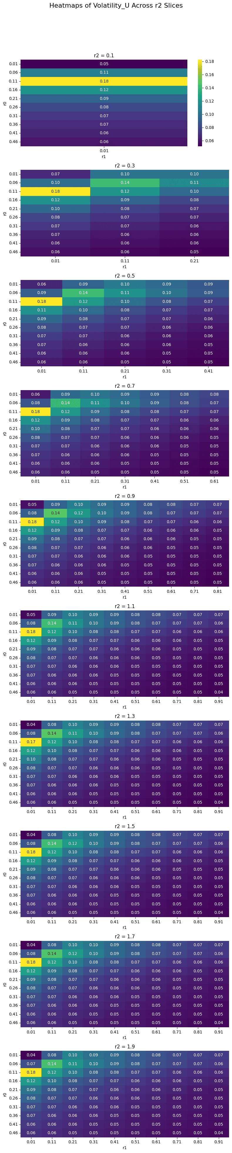
The volatility of the rate reduces as r0 and r1 diverge, and increases at higher levels of divergence. r2 seems to amplify the volatility, which makes sense as the maximum rate values spike higher.

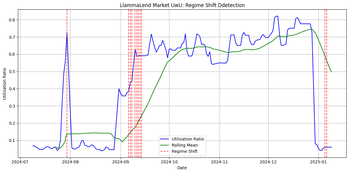
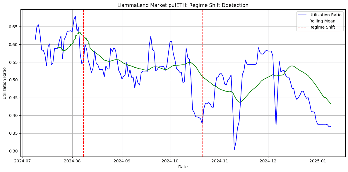
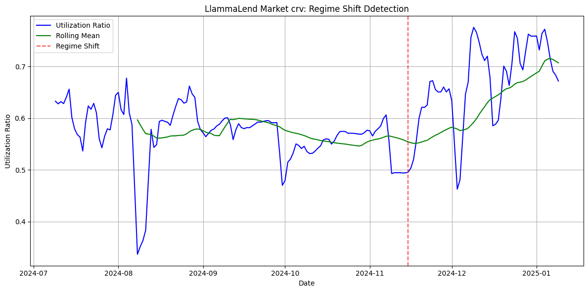
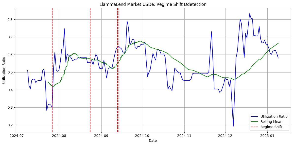
A.2 Re-parameterisation Framework

Our model is limited to stationary periods in utilization rate, which generally are associated with a demand for a given asset and depend on rates and availability on alternative lending markets.

We use a simple rolling statistical approach based on z-scores. We process the utilization rate to identify significant deviations. It calculates the rolling mean and standard deviation over a specified window (default: 30 days) and computes z-scores to measure deviations from the rolling mean. A threshold-based approach is applied, where utilization ratios exceeding an absolute z-score threshold (default: 1.5) are flagged. To confirm a regime shift, deviations must persist for a predefined number of consecutive days (default: 7), reducing false positives.

Regime shifts tend to be identified in a range of 1-4 month intervals, indicating a rough timeline of the frequency that re-parameterization may be advisable. Below we show the results for the different lending markets:

A.3 Validating Impact of Parameter Changes

We can utilize an Event Study Methodology with 3-tiered control and multiple windows designed to measure the short-, medium-, and long-term effects of a parameter change (e.g., interest rate curve update) in a decentralized lending market. It compares a treated pool against a control chosen using a 3-tiered approach:

1. a nearly identical direct control pool,

2. a weighted composite control with difference-in-differences (DiD), or

3. a broad market index when neither of the first two is available.

The impact is assessed over three post-change windows—short-term (e.g., 7 days), medium-term (e.g., 30 days), and long-term (e.g., 60–90 days)—to distinguish immediate reactions from persistent shifts. Key metrics include utilization ratio, borrow/supply amounts, and optionally, volatility measures.

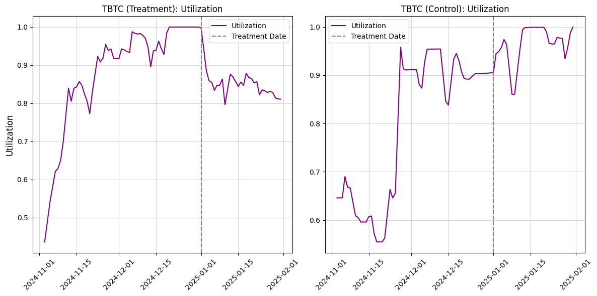
A.3.1 Example: tBTC Parameter Changes for a Direct Control Pool

In order to test the framework, we analyze changes to monetary policies on LlamaLend Markets in the past. We specifically focus on the recent proposal to change min and max rates on Arbitrum. For demonstration purposes, we focus specifically on the tBTC market. The transaction to execute parameter changes took place on 01-01-2025.

Market Details

• Treatment Pool - tBTC market (Arbitrum)

• Control pool - tBTC market (Mainnet)

Utilization

For the metric utilization, a Paired t-test was conducted to test whether the post-treatment values were greater than the pre-treatment values. The Shapiro-Wilk test for normality yielded a p-value of 0.4879, indicating that the differences are normally distributed. The Paired t-test produced a test statistic of 8.9255 and a p-value of 0.0001. The result is statistically significant at the 5% level, supporting the alternative hypothesis.

Borrow/ Supplied

For the metric total_assets_usd, a Paired t-test was conducted to test whether the post-treatment values were less than the pre-treatment values. The Shapiro-Wilk test for normality yielded a p-value of 0.6634, indicating that the differences are normally distributed. The Paired t-test produced a test statistic of -9.1148 and a p-value of 0.0000. The result is statistically significant at the 5% level, supporting the alternative hypothesis.

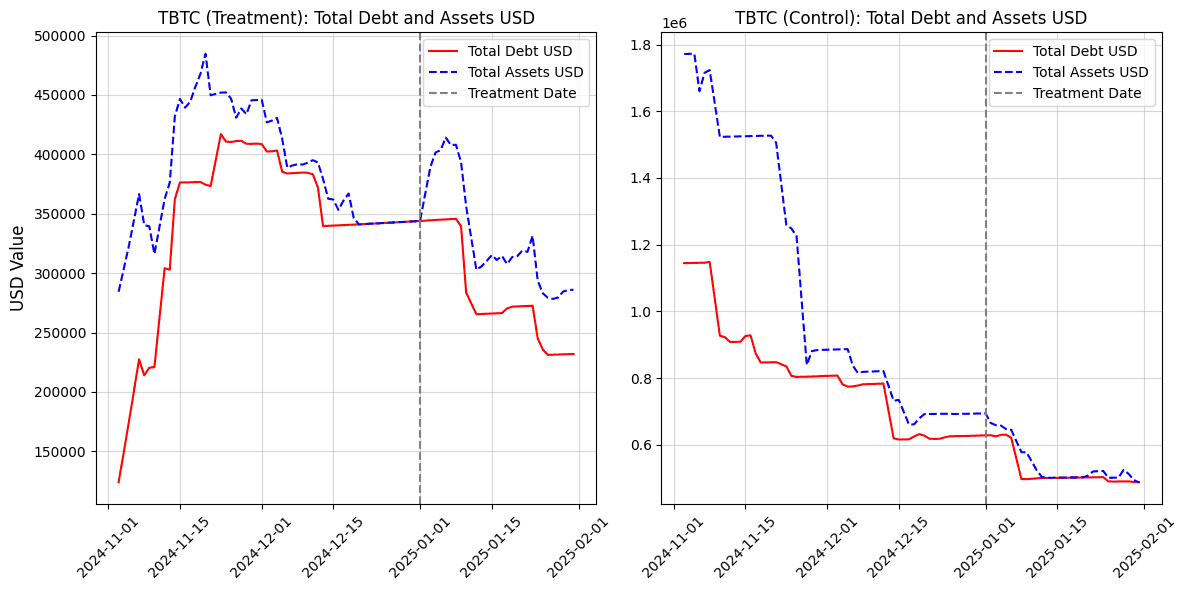
For the metric total_debt_usd, a Wilcoxon Signed-Rank Test was conducted to test whether the post-treatment values are different from the pre-treatment values. The Shapiro-Wilk test for normality yielded a p-value of 0.0012, indicating that the differences are not normally distributed. The Wilcoxon Signed-Rank Test produced a test statistic of 3.0000 and a p-value of 0.0781. The result is not statistically significant at the 5% level.

A.4 Succinct Overview of the Literature

For further reading, a selection of relevant literature with sources is provided.

Interest Rate Models (IRMs) in DeFi lending protocols, such as those used by Aave and Compound, often rely on static or piecewise-linear interest rate curves tied to utilization rates. While effective in ensuring liquidity, these models often lack the flexibility to respond dynamically to market conditions.

Recent advancements include the adoption of adaptive frameworks, such as PID controllers and stochastic optimization. Bastankhah et al. (2024) introduced a dual-component IRM combining rapid rate adjustments with long-term risk optimization, while Bertucci et al. (2024) formulated optimal control-based IRMs that outperform linear designs in high-utilization scenarios. Boneh (2024) highlighted the practical efficiency of PID-based systems for real-time utilization adjustments.

Challenges such as market segmentation, exploitation vulnerabilities, and equilibrium inefficiencies remain. Chitra et al. (2023) documented attack vectors like recursive borrowing, emphasizing the need for elastic rate adjustments and robust parameter tuning. Chaudhary et al. (2023) highlighted the weak integration of DeFi IRMs with broader market dynamics, calling for off-chain data incorporation.

The literature underscores a trade-off between stability, efficiency, and security. Promising directions include elastic IRMs, hybrid control frameworks, and data-driven parameter optimization to ensure adaptability, resilience, and practical applicability in dynamic DeFi markets.