Useful Links:

• Website: defi.money App

• Documentation: Docs | GitHub

• Social: defi.money Twitter | Blog

• Related Work: LlamaRisk Initial Parameter Recommendations | LlamaRisk Methodology Explainer

• Dashboard: defi.money Risk Portal

Section 1: Executive Summary

This section introduces the scope and goals of our research and provides a summary of results for convenient access.

1.1 Executive Summary

DeFi.money is a Layer 2-focused stablecoin platform inspired by the crvUSD protocol. It enables borrowers to mint the MONEY stablecoin from a diverse array of collateral assets. The platform employs the innovative Lending Liquidating Automated Market Maker Algorithm (LLAMMA) from Curve to rebalance borrowers' collateral and facilitate the progressive, bi-direction liquidation of their positions. This mechanism, referred to as soft-liquidation, mitigates the need to fully liquidate borrower positions unless necessary.

DeFi.money carries risks inherent to traditional lending platforms, particularly the risk of missed liquidations, which can occur due to insufficient liquidity and excessive price volatility. Additionally, it faces unique risks associated with the crvUSD architecture, such as the accumulated loss from collateral rebalancing, incurred to the borrower.

This report focuses on evaluating these risks under various stress scenarios by conducting simulations of different market stress severity using an agent-based simulator based on Xenophon Labs' work. The ultimate objective is to provide quantitative guidelines on selecting assets for onboarding and to determine the optimal parameters for markets utilizing such collateral.

1.2 Results Summary

Below are the updated recommended parameters for defi.money collateral assets based on our advanced ABS model output. The values below are refined parameters that we had previously provided in our initial recommendation report, which was based on LLAMMAsimulator by michwill.

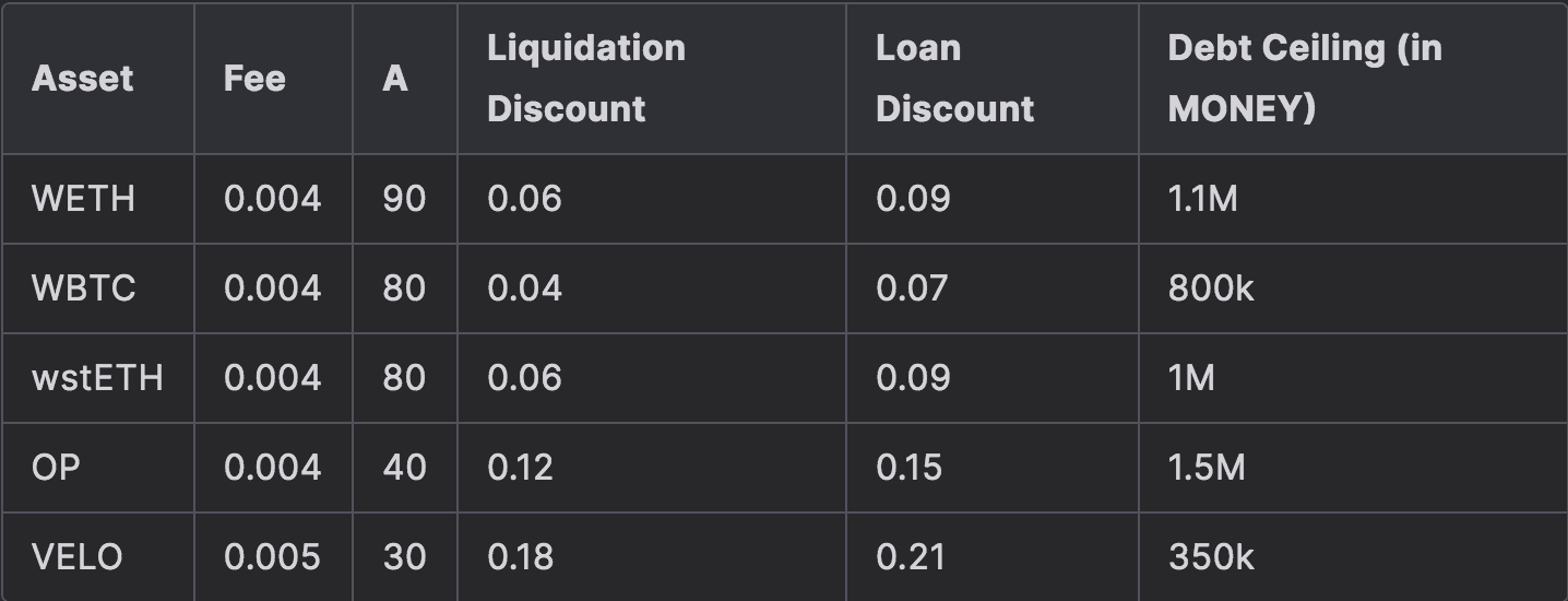
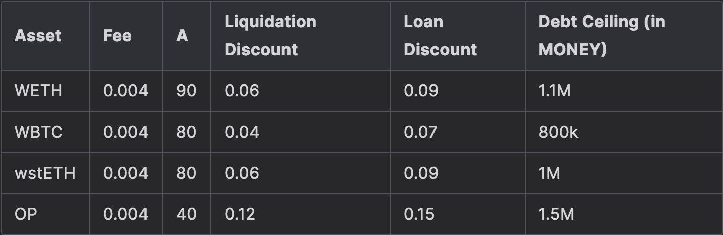
Recommended parameterization for collateral tokens on Optimism

Recommended parameterization for collateral tokens on Arbitrum

We provide recommendations based on the simulation results in Section 5 of this report.

Section 2: Background

This section provides an overview of how we approach optimizations based on the protocol design, understanding relevant parameters, and quantifying risk metrics. The background information outlined here informs our risk model methodology in the subsequent section.

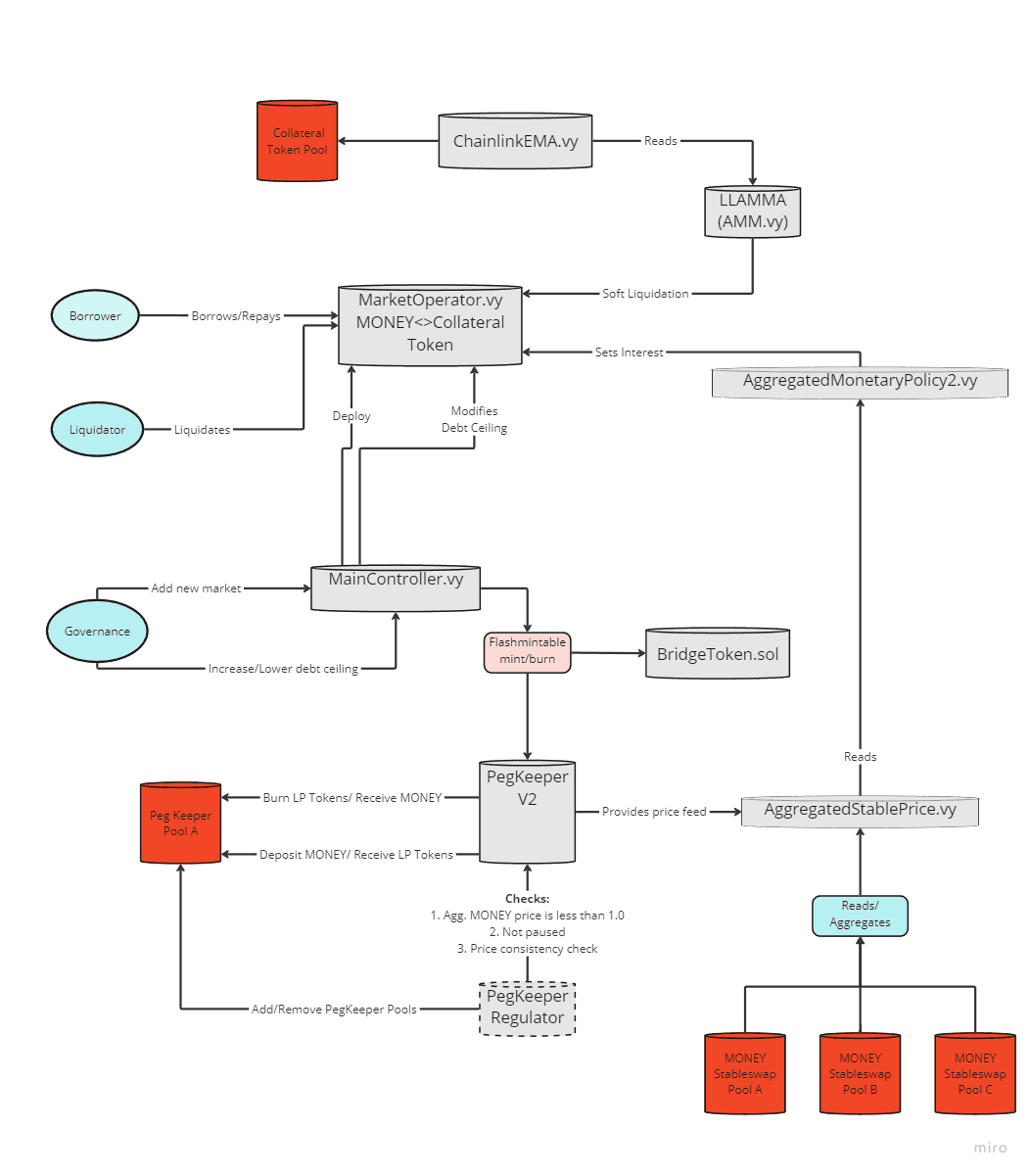
2.1 Defi.money Architecture

MONEY is a USD-denominated decentralized stablecoin designed for cross-chain interoperability across EVM blockchains, optimized for Layer 2 environments such as Optimism, Arbitrum, and Base.

This stablecoin utilizes a collateralized debt position (CDP) model, allowing users to mint MONEY using a variety of collateral types, including altcoins and tokenized real-world assets.

The underlying protocol, built on the Curve Finance crvUSD architecture, protects the borrower from collateral price volatility through a soft-liquidation process that automatically rebalances borrow positions between MONEY and collateral asset. It is based on the LLAMMA system, here renamed the "Automated Loan Protection" system.

The Automated Loan Protection system enhances the protocol by managing collateral automatically through a lending and liquidating automated market maker (AMM) algorithm. This ensures that users are protected from short-term price volatility while providing a low-cost means of value transfer.

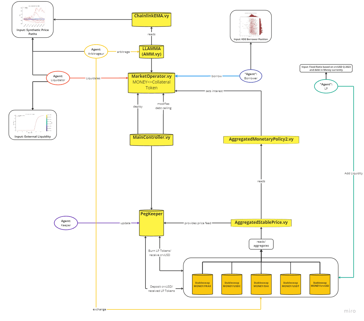
We provide an overview of the protocol architecture below.

2.2 Asset & Parameter Scope

2.2.1 Asset Scope

The following assets on the respective chains are included in the scope of this analysis:

• Optimism | $WETH, $WBTC, $wstETH, $OP, $VELO

• Arbitrum | $WETH, $WBTC, $wstETH, $ARB, $GMX, $PENDLE, $RDNT

These assets can be split into two categories. Firstly, we have a batch of assets that have a history of being used as collateral in the crvUSD protocol (WETH, wstETH, WBTC). The other batch requires additional care (e.g. ARB) since little to no data is present. The latter, comprising governance tokens with substantially less market maturity and more price volatility, present a greater risk.

2.2.2 Parameter Scope

The simulation tool will allow us to make informed recommendations for market parameters based on the historical behaviors of each asset in adverse scenarios. These parameters stay constant during the life cycle of a market. Correctly selecting these parameters is essential to the overall health of a given market, and has repercussions for the protocol as a whole. Conversely, an improper choice of parameters adds friction to the liquidation mechanism and increases the risk of accumulating bad debt. Here is the list of market parameters that we will optimize for:

• A: The amplification coefficient defines the liquidity density and band size. The relative band size is 1/A.

• Fee: AMM fee in the market's AMM, which is charged on token exchanges.

• loan_discount: The percentage used to discount the collateral for calculating the maximum borrowable amount when creating a loan (i.e. the buffer between max loan-to-value and liquidation threshold).

• liquidation_discount: Discount defining a liquidation threshold.

• debt_ceiling: max stablecoin debt that can be minted within the market.

We know these parameters depend overall on the collateral's volatility as well as the liquidity of both MONEY and the collateral. However, only an agent-based simulation, as described in Section 3, will give us a quantifiable outline of this dependence.

2.2.3 Parameterization Significance

We emphasize the importance of carefully selecting market parameters. From this point forward, we will refer to the "equilibrium value" as the optimal parameter value in a specific context. For the time being, we will not define the precise concept of optimality.

1. liquidation_discount: If the parameter value is below the equilibrium value, there are fewer incentives for the liquidator to close an unhealthy position. Positions with excessively large debt may not be liquidated due to the high price impact, and there may not be enough margin for the initial liquidator to close the position before it becomes undercollateralized. Conversely, if the parameter value is above the equilibrium value, the borrower may incur excessive losses.

2. loan_discount: In a DeFi money market, the loan discount is utilized to determine the maximum loan-to-value (LTV) ratio of a Collateralized Debt Position (CDP), which represents the maximum proportion of collateral that can be converted into debt. If the loan discount is above the equilibrium point, unnecessary hard liquidations may occur due to oracle volatility. Conversely, if it is below the equilibrium point, the system will be capital inefficient.

3. debt_ceiling: The debt ceiling is intrinsically dependent on the available liquidity of the MONEY token and the collateral token. If the debt ceiling is set higher than the equilibrium point, the debt will not be liquidated effectively because the price impact of trades associated with the liquidation exceeds the discount on the collateral. Conversely, if the debt ceiling is set lower than the equilibrium point, the market will not reach its full potential.

We note that a conservative approach can always be taken when selecting the aforementioned market parameters, which does not require advanced simulations. While conservative parameter values do not pose significant risks to the health of the system, they do result in inefficiencies. The goal of the simulation tool is to maximize system efficiency while mitigating the primary risk vectors within a lending market. The next section provides a more detailed examination of these risk vectors.

2.3 Risk Vectors

This work focuses on standard risks in lending markets, all related to protocol solvency. The primary goal will be therefore to provide empirical guarantees of overcollateralization at all times.

2.3.1 Bad Debt

Given a certain lending market, i.e. a collateral token against which one can borrow MONEY, unhealthy positions might fail to be properly liquidated. This is caused by either large price fluctuations of the collateral or insufficient liquidity. Insufficient liquidity can be manifested in two ways:

1. Insufficient Sell-Side Liquidity: There isn't enough sell-side liquidity for defi.money, hindering liquidators from repaying a Collateralized Debt Position (CDP) debt.

2. Insufficient Buy-Side Liquidity: There isn't enough buy-side liquidity for the collateral token, making it difficult for liquidators to sell the received collateral at a profit.

Undercollateralized CDPs are aggregated into a metric called bad debt, which refers to MONEY debt from accounts with sub-zero health. The primary risk metric is the maximum amount of bad debt observed in each simulation, with evaluations based on mean, median, and p99 values across all simulations. The p99 bad debt metric, which is analyzed over a 24-hour simulation horizon, represents the worst-case daily scenario.

Uncontrolled growth of bad debt leads to protocol insolvency, where the aggregate value of debt exceeds the aggregate value of collateral. This in turn entails the risk of MONEY losing its peg.

2.3.2 Cascading Liquidations

Liquidation of unhealthy CDPs may have a non-negligible impact on the prices of the collateral asset and MONEY whenever the debt of the CDP is significant compared to the available liquidity. Liquidating a CDP requires the acquisition of MONEY token and the sale of the collateral token. These actions push the value of the collateral token, denominated in MONEY, downwards. In turn, this price shift might cause other CDPs to become eligible for liquidation.

This phenomenon is modeled by using the price impact curves of each Pegkeeper pool. Hence, a large acquisition of MONEY will cause the collateral price to decrease, potentially triggering further liquidations in the system.

However, since price trajectories of collateral assets are treated as exogenous to the system, we do not model the price impact of collateral sale during the liquidation process. This is a limitation to the current framework since it dampens the effect of liquidating large positions in the system.

The assumption remains reasonable so long as two cases are satisfied:

1. The buy-side liquidity of MONEY is significantly smaller than the sell-side liquidity of the collateral token, causing the impact of the liquidator on the market's oracle to be concentrated MONEY acquisition.

2. The debt ceiling is carefully chosen with respect to the sell-side liquidity of the collateral so that liquidation of all the debt inside of a market does not impact collateral price.

2.4 Metrics

The metrics for the simulation are succinctly summarized and captured in the table below:

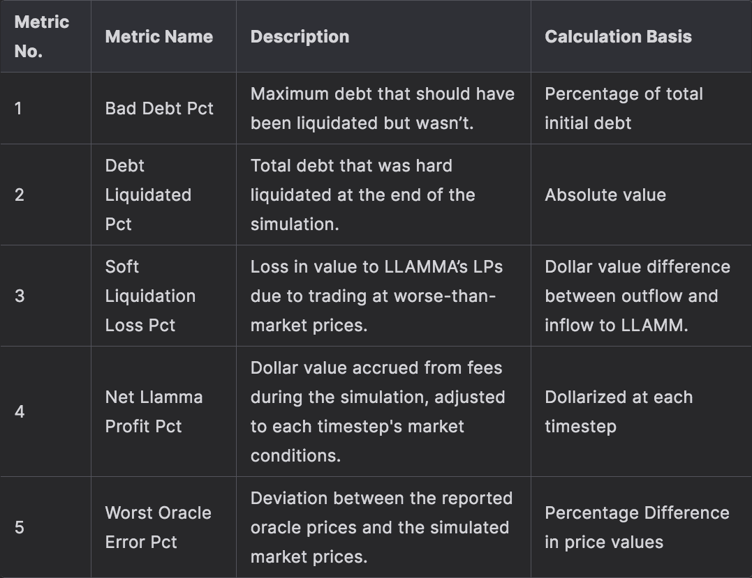
Aggregation: Metrics are aggregated across all simulations, focusing on mean, median, and p99 values.

Normalization: Bad Debt, Revenue, and Fee metrics are normalized as a percentage of total initial debt to compare across different scenarios.

Price Marking: For Revenue and Fee metrics, the simulated Aggregator price is used as a dollar equivalent for MONEY.

Section 3: Risk Model Overview

This section describes the methodology and components that make up the simulation. It covers the foundations of our research work and details the inputs and agents that compose the simulation.

3.1 Simulation Strategies

The model leverages three prevalent financial risk management strategies:

1. Agent-Based Modeling: model key rational agents' actions on Defi.money smart contracts and capture the result of the overall interactions.

2. Stress Testing: market stress is expressed in three components: collateral price volatility, low liquidity, and low debt collaterization

3. Monte Carlo simulations: take snapshots of relevant metrics over large number of runs to capture the average and extreme outcomes.

Together, these strategies involve running numerous simulations to evaluate system performance under different stresses, each spanning 24 hours with updates every five minutes, balancing computational efficiency with accuracy. This setup helps predict how Defi.money’s smart contracts will respond to dynamic market conditions.

To model the system smart contracts, we rely on curvesim and crvUSDsim. Both packages offer Python classes for interacting with Curve smart contracts. For instance, we can simulate the precise impact of an arbitrageur’s trade on MONEY prices by modeling the underlying LLAMMA pool directly. We have also modified the crvUSDrisk package as a foundation for generating parameterizations for existing markets.

Note: We base our work on Xenophon Labs, who have build a robust simulation tool to model overall system risk of crvUSD. We also made us of nomenclature and explanations used by Xenophon in this report and acknowledge their contribution.

3.2 Model Inputs

See the architecture of the simulation components below:

3.2.1 Prices

We model collateral prices through Geometric Brownian Motion (GBM) processes and employ Ornstein-Uhlenbeck (OU) stochastic processes to simulate stablecoin prices (they are traditionally used to model the trajectories of instantaneous interest rates). For more information about the mathematical modeling of financial markets, we refer to Martingale Methods in Financial Modeling, M.Musiela & M.Rutkowski. The main property of the latter family of processes is that they are mean-reverting, that is the trajectories tend to concentrate around a constant. This constant would be 1 in the case of stablecoins. The brief deviations from the mean therefore model depeg scenarios of varying severity.

For the Flash crash scenario (see Stress-test Scenarios for Dashboard), we simulate correlated asset prices, which is relevant given that crypto-asset prices are generally correlated. This can especially be observed during highly bearish market tendencies. In addition, we incorporate jumps to the above processes to model aggressive buy/sell movements inside of the market.

The processes parameters, such as the drift, instantaneous volatility, and the mean-reverting speed (in the case of OU processes), are calibrated using up to four years of empirical price data, whenever it is available.

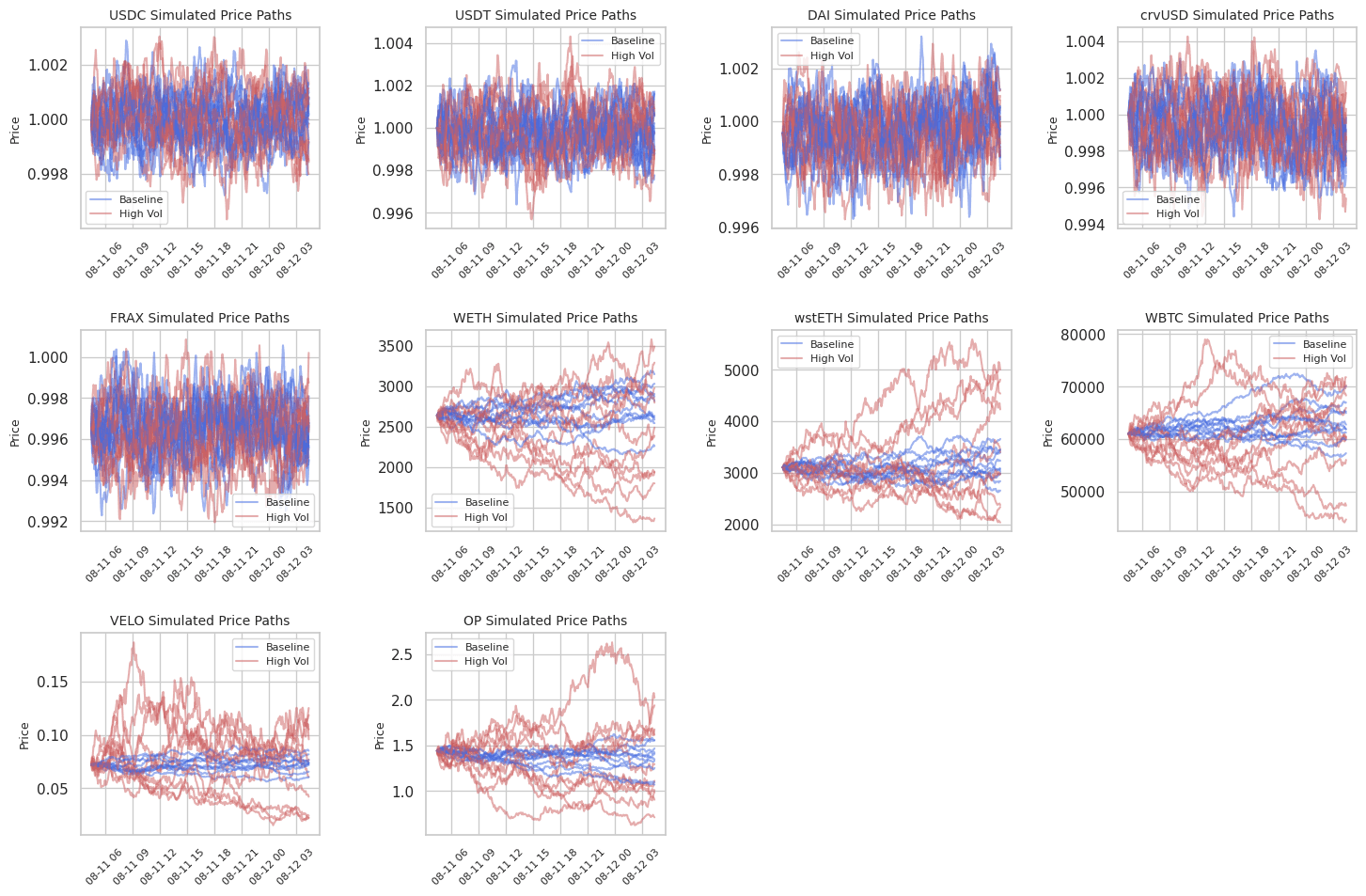
Below we show, as an illustrative example, generated price trajectories for some assets on Optimism. We present two scenarios:

• the baseline scenario (blue) and

• the high volatility scenario (red),

where the volatility parameter is chosen 1.5x worse than the 99th percentile of the realized volatility distribution.

3.2.2 Debt

In our simulations, we treat borrowers as passive participants. At the beginning of each simulation, we sample borrower positions from a learned debt distribution upon meeting a preset debt threshold. The dynamics of debt will then be driven by price fluctuations between collateral and MONEY as well as the action of agents in the system.

Passivity of borrowers is a conservative approach, implying borrowers will not proactively repay their debt, thereby increasing the reliance on liquidators to maintain system solvency. This assumption is reasonable for our 24-hour simulation window.

Each simulation begins by generating a debt distribution that reflects realistic conditions. This is achieved by sampling historical user data from the crvUSD controllers and Llamalend market whenever possible. For synthetic markets, we parameterize based on the borrower distribution from other lending markets.

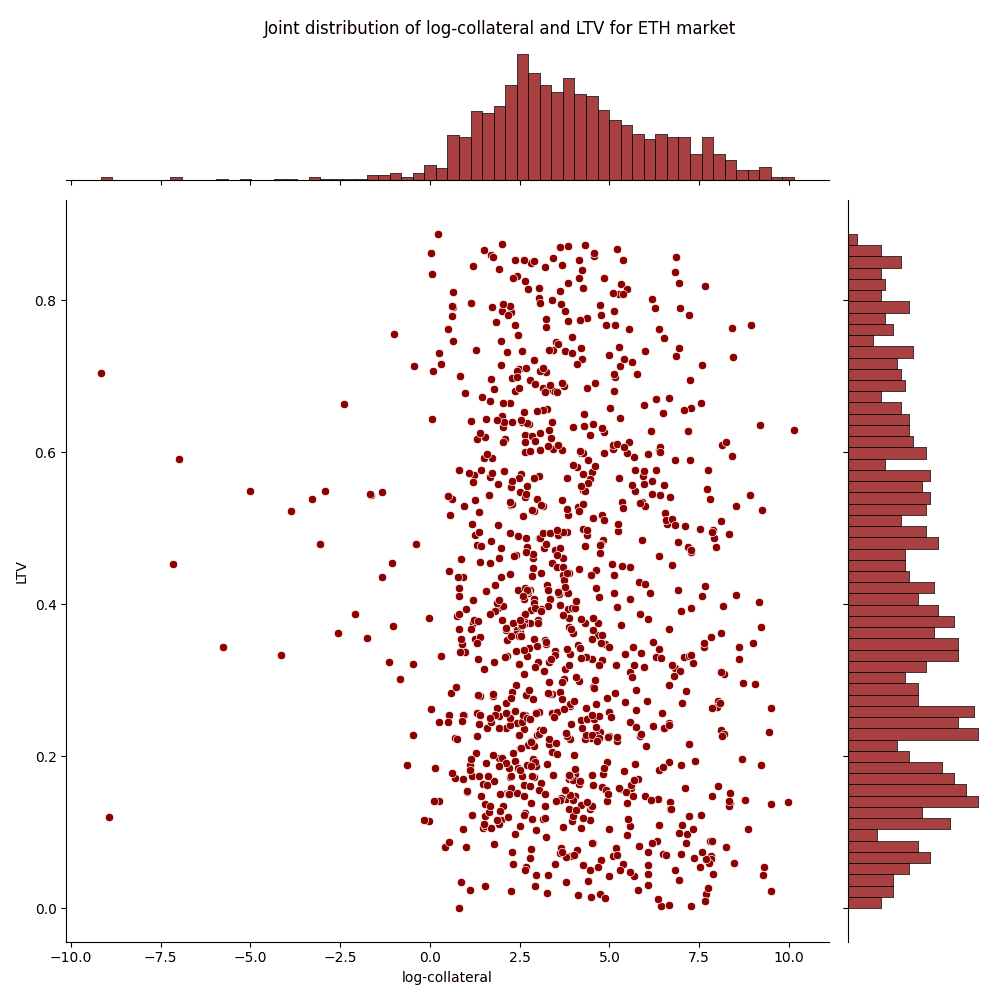
More specifically, the state of a passive borrower position at a given point in time is described by the amount of collateral token and the amount of borrowed token, which stay constant during the simulation, and the exchange rate between the collateral token and MONEY, which is dynamic in time. At each point in time, the state of the borrower's position is treated as an independent sample. We gather these samples into an aggregate dataset for each relevant market. The risk of a borrower's position is quantified using the loan-to-value metric, which is the ratio of debt and the collateral denominated in the same numéraire.

We then use a Gaussian Kernel Density Estimator (KDE) to model realistic debt levels by focusing on the health of a position. We create a position with bands that would reflect the health of a sampled position by reverse engineering the number of bands that would represent the health of the position. The major advantage of this is it works great to transfer the empirical distribution from the lending market into the simulation environment, but also allows us to use data from other lending markets to calibrate initial debt distributions.

Finally, new loans are sequentially created until a preset debt threshold is reached.

Below we show the joint distribution of the log-collateral of sampled borrower positions and their associated LTV for the WETH market.

3.2.3 Internal Liquidity

Internal liquidity refers to the aggregate liquidity without MONEY Pegkeeper pools. As the ratio of MONEY debt to available MONEY liquidity in these pools increases, liquidating the current debt has a significant price impact on the market. In particular, it can adversely affect the peg of MONEY, propagating possible liquidations to other markets.

For our simulations, we use current liquidity from the StableSwap pool and initialize debt relative to this. We model the liquidity of each pool —for instance, the amounts of USDC and MONEY in the MONEY/USDC pool— using a multi-variate normal distribution derived from empirical data.

These amounts are then adjusted to achieve the desired debt-to-liquidity ratio for the simulation. For example, with a 2:1 debt-to-liquidity ratio and an initial simulation setting of 100M MONEY in debt, we ensure that the liquidity sampled in the Pegkeeper pools amounts to a total of 50M MONEY in deposits.

3.2.4 External Liquidity

For the broader context of our simulations, the external liquidity for each collateral asset is modeled using a price impact curve. This curve begins at zero for infinitesimally small trades and asymptotically approaches a 100% impact as trade size increases.

This relationship is captured through regression analysis on historical trading data, which was sourced using APIs from ParaSwap and KyberSwap for various MONEY trading pairs. The data covers a wide range of trade sizes from 100 USD to 50 Million USD, allowing us to construct an empirical slippage curve for these assets.

We then use an isotonic regressor to model the slippage curves. Isotonic regressors have the property to yield non-decreasing predictions, i.e. the larger the trade, the higher the price impact.

Below we extract the Price impact quotes for swapping OP into crvUSD from the 9th of August, as well as the fitted model.

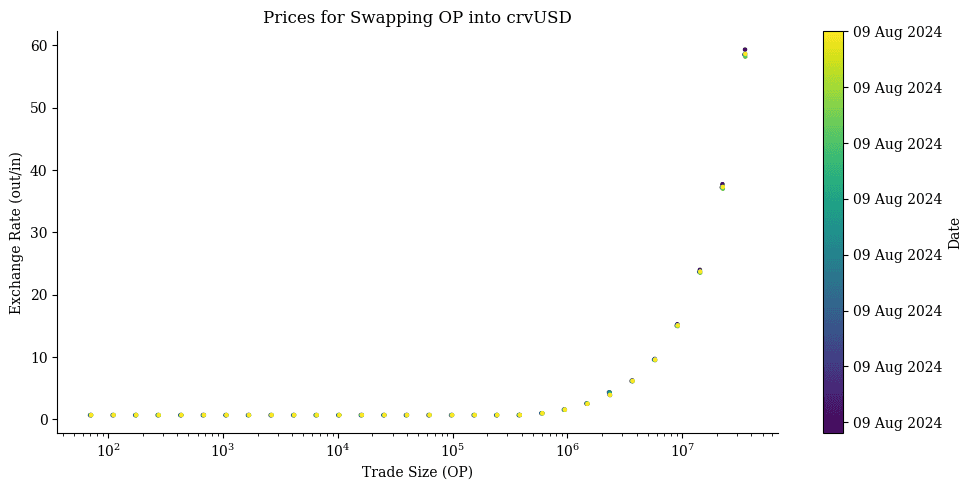
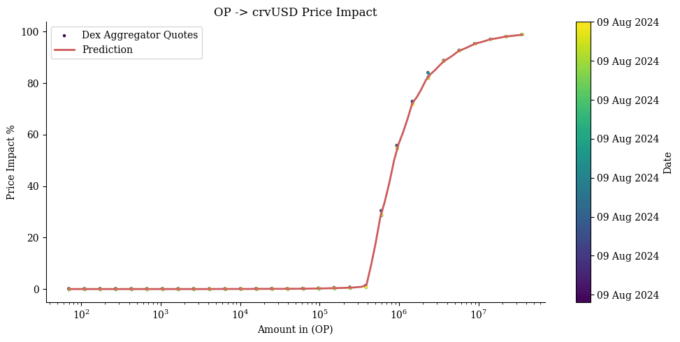
We can see that liquidity dries up at around 1,000,000 in OP swapped into crvUSD.

Note: We track swapping quotes dynamically. This enables us to offer warning systems if liquidity should change based on market conditions. This allows us to give updated recommendation as needed for debt ceiling defined in the controller of the respective MONEY collateral markets. Future work could include to track additional lending markets. The benefit of this is to estimate liquidation volume across protocols which currently is not accounted for and may affect the ability of liquidators to liquidate unhealthy positions in the defi.money system.

3.3 Agents

In our simulation, agents trigger state transition along with price dynamics of the collateral against MONEY. The simulation models the action of three agents:

1. the keeper,

2. the arbitrageur and

3. the liquidator.

Note that since we make the assumption of passive borrowing, we shall not model the borrower as an agent.

3.3.1 Keeper

The keeper adds/removes MONEY from the Pegkeeper pools whenever doing so is profitable. It does so by calling the update() function. More specifically, it adds liquidity to the pool whenever MONEY trades above peg, and removes liquidity whenever it trades below peg.

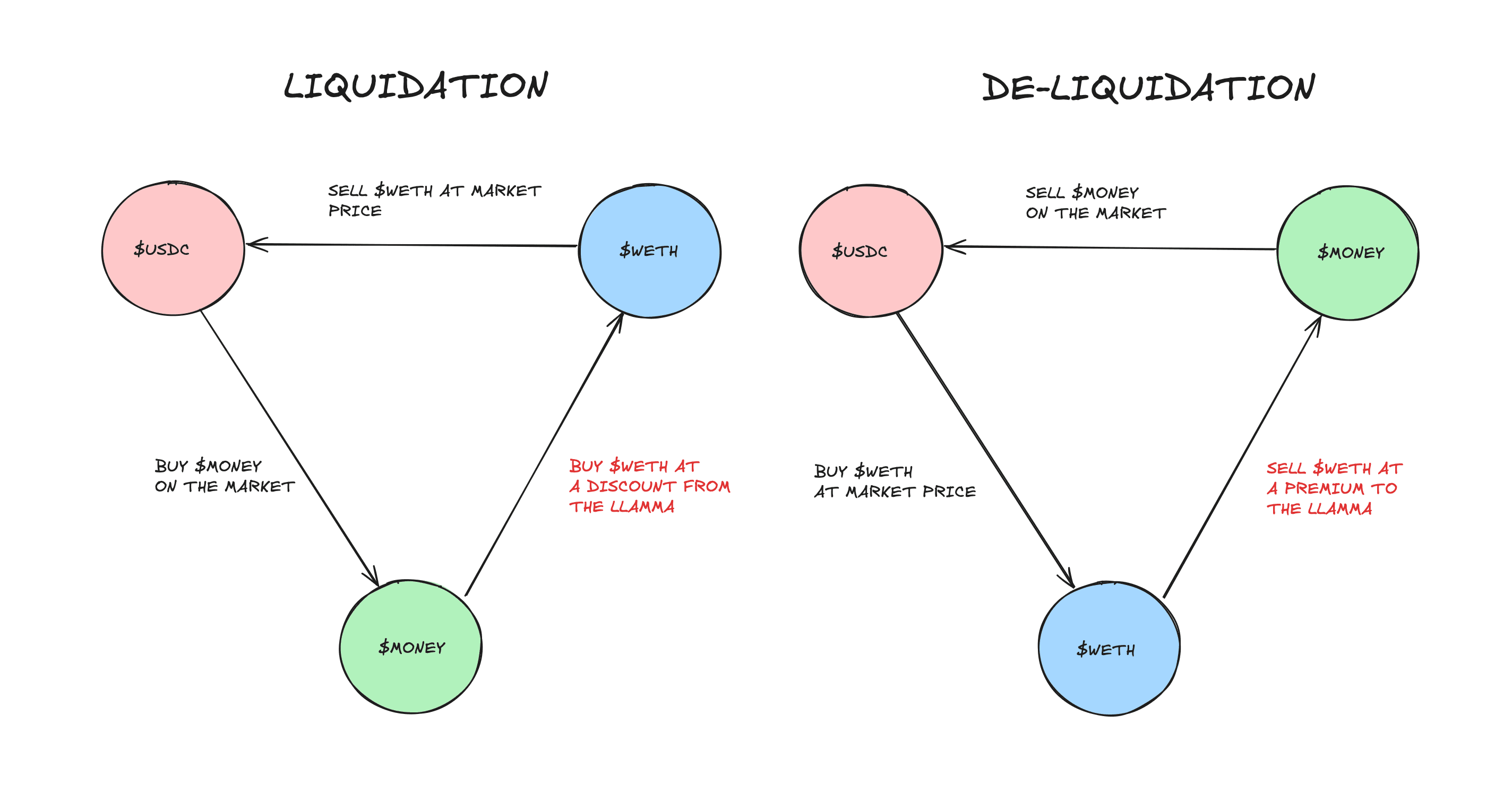
3.3.2 Arbitrageur

The arbitrageur ensures soft-liquidation of the borrowers' positions in exchange for profit. It rebalances between collateral and MONEY at a better than market price, due to the structure of the LLAMMA algorithm. The LLAMMA is an AMM that offers better-than-market prices to incentivize arbitrageurs to rebalance the collateral of a borrower's position. It does so by quoting the collateral lower when the prices decrease and higher when the prices increase.

Arbitrageurs can then partially liquidate borrower's positions when the collateral price decreases, and partially de-liquidate when the collateral price increases, in exchange for profit. The spot profit is determined by the difference between the market price and the LLAMMA quoted price. In reality, market friction has to be taken into account.

We model the arbitrageur action as the execution of optimal arbitrages of cycle length 3. In the case of liquidation, the arbitrageur purchases MONEY, buys the borrower's collateral at a lower-than-market price, and sells it on the market. In the case of de-liquidation, the arbitrageur purchases the collateral token on the market, exchanges it for MONEY at higher-than-market price, and sells the latter token on the market.

Here is an illustrated example of the arbitrageur's action on a MONEY/WETH market. Let x be the initial amount of $USDC and f(x) be the terminal amount of $USDC obtained after traversing one of the cycles depicted below. The arbitrageurs seek to find x such that f(x) - x is maximized. If f(x) - x > epsilon, where epsilon is some profitability threshold, the arbitrageur will execute the trade in the simulation.

3.3.3 Liquidator

The liquidator ensures the hard liquidation of borrowers' positions whenever they are eligible. Hard liquidation occurs whenever the loan-to-value ratio exceeds the maximum debt threshold, which depends on constant market parameters (amplification coefficient and liquidation discount), as well as the number of bands over which the position is spread.

When a position is eligible for hard liquidation, the liquidator repays the debt of the position in exchange for the discounted collateral, if it is profitable to do so. In more detail, if it is profitable, the liquidator purchases MONEY, pays back the debt of the position, receives the discounted collateral, and sells it on the market. Note that the health of the lending market is highly dependent on both the available MONEY and collateral asset liquidity.

3.4 Market Stress Testing

The primary purpose of the agent-based simulation is to parameterize MONEY markets. For this, we designed edge-case scenarios that test the market in adverse scenarios and evaluate the parameterization on the overall system behavior. The scenario is often not characterized by realism but designed to identify how the respective MONEY market behaves in the context of the overall system under extreme conditions. For the dashboard we conversely simulate the overall MONEY system under realistic conditions and try to simulate the overall health rather than that of the individual collateral market.

We focus on three primary sources of market stress:

• Price volatility: The expected variance in asset returns.

• Debt: The initial amount of debt in the system at the start of the simulation.

• Liquidity: The amount of MONEY liquidity available for liquidations.

3.4.1 Volatility

We analyzed the intraday volatility for all collateral assets since inception except for assets older than 2020 (such as ETH and BTC), where we capped the analysis horizon to January 2020. For this, we annualized the standard deviation of log on a rolling 24-hour basis.

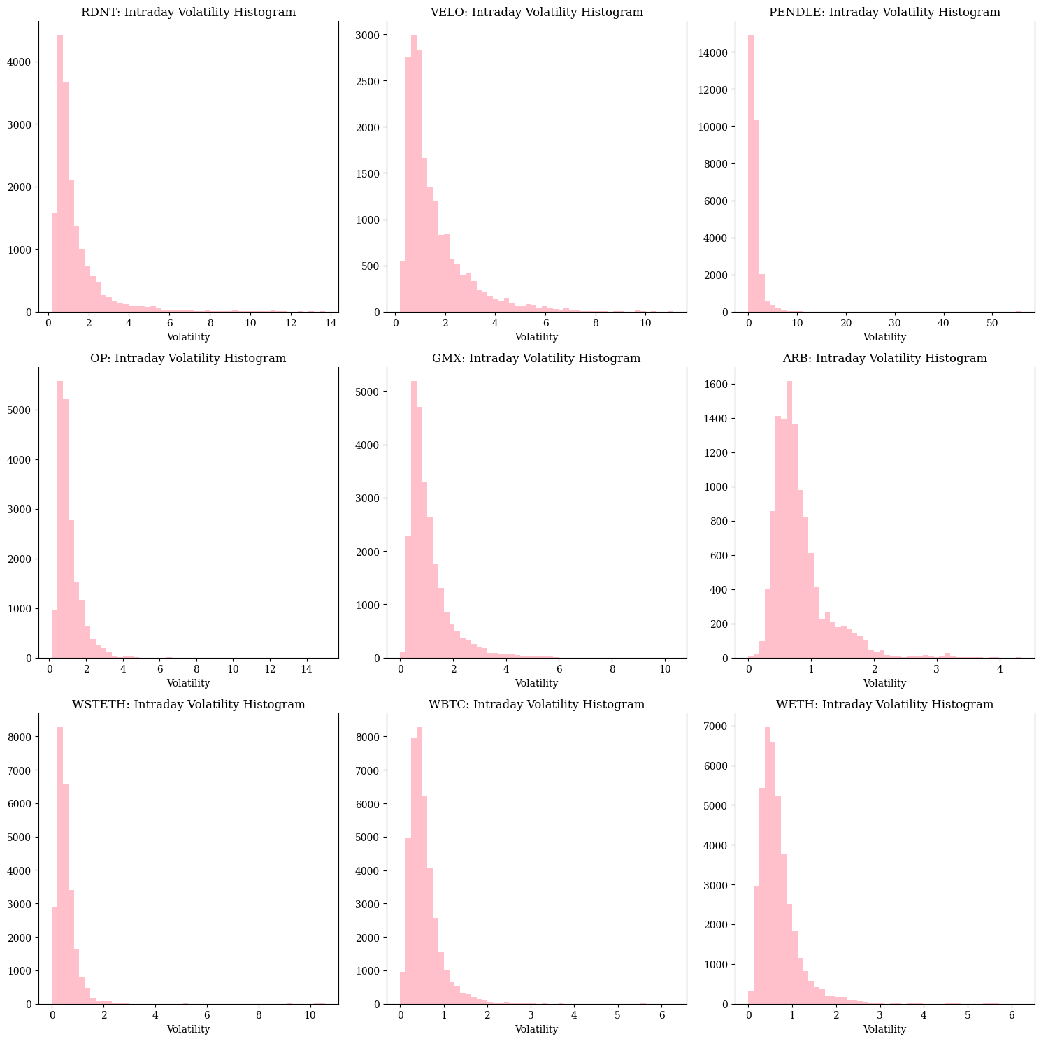
Our parameterization stress-test scenario is characterized by volatility that is 1.5 times worse than the 99th percentile of observed volatility. The design rationale for this scenario particularly considers newer assets, which tend to be more volatile and have less available price history, thereby necessitating additional caution. A recent severe volatility event in early August 2024 exemplifies this point, where previous simulation tools (and the one utilized in the initial recommendations for defi.money markets) were unable to adequately account for unprecedented volatility which has led to a modest 0.1% in bad debt in ETH markets.

3.4.2 Debt & Liquidity

MONEY liquidity is currently concentrated in the Pegkeeper pools and, given crvUSD as an example, it is likely to remain concentrated there. In previous research, a relatively stable debt-to-liquidity ratio was found for crvUSD, ranging from 2:1 to 3:1 (Xenophon, 2024). For the parameterization example, we set the Debt:Liquidity Ratio fixed on this ratio. The Liquidity values in MONEY are fetched from the current Pegkeeper pools per chain from DeFi.money. This makes sense as liquidity is extremely thin in Pegkeeper pools making it ideal for simulating an adverse liquidity scenario. The debt is matched based on the fixed ratio. The distribution of debt is maxed out in valid borrower positions initialized from the borrower model (see Section 3.2.2) collateral token that we are trying to parameterize. This liquidity is unlikely to be observed, however, given we are trying to be prudent in the parameterization of markets, it is ideal for stress testing.

Method: Debt ceiling for collateral assets (outside of simulation scope)

We define the debt ceiling for the respective markets outside the scope of the simulation. This decision is based on the fact that, while we can estimate liquidation volume originating from DeFi.money, we cannot estimate liquidation volume from other platforms. Therefore, we adopt a conservative approach and identify the maximum instantaneous trade size that can occur without causing significant price impact when a liquidator swaps from a collateral asset into a major stablecoin (i.e. USDC, USDT), identifying the points where liquidity starts to diminish based on DEX quotes.

For this, we simulate trades for collateral assets into USDC/USDT, fit an Isotonic regressor onto the shared quotes, and identify the largest rate of change in liquidation impact capped between 3% to 20% price impact. The rationale for this is that if we remain within the maximum instantaneous trade size, i.e. the trade size which allow to swap an asset with reasonable slippage, we could theoretically liquidate the entire collateral in a DeFi.money market, assuming liquidity conditions remain stable.

While this may sound overly conservative, as profitable liquidations can happen at higher slippage levels and swapping into alternative (stable) assets (apart from USDT and USDC) can occur, we know liquidity conditions can change drastically in volatile periods. This is due to liquidation volume for the same assets from other DeFi protocols and LPs leaving pools to escape volatility. Hence, we believe it is a balanced trade-off.

3.4.3 Summary of Scenarios

We simulate the Defi.money system as if it were run on one market. We initiate our scenario as follows:

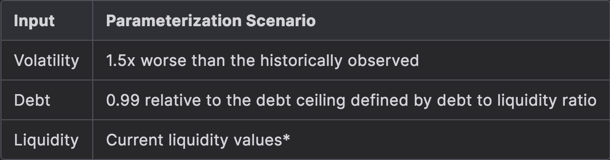
*Given that Liquidity right now can be considered severe - there is no reason to induce severe liquidity conditions.

Section 4: Results

This section shares the analysis of the simulation output for all assets in the scope, which allows us to form recommendations for optimal parameters. We also share our analysis to determine suitable debt ceilings.

4.1 Market Parameters

We ran for each asset through the simulation. For each asset we defined "unsafe runs" as those that resulted in Bad debt in p99 scenario, which were consequently removed from the analysis. After this we followed the simple algorithm to maximize Net Llamma Profit Pct Median and minimize Soft Liquidation Loss Pct Median, Borrower Loss Pct Median,Worst Oracle Error Pct Median using the Tchebycheff Method.

The Tchebycheff method in multi-objective optimization focuses on minimizing the maximum deviation of objectives from their ideal values, ensuring a balanced trade-off among conflicting goals. By concentrating on the worst-performing objective, it prevents any single objective from performing disproportionately poorly, making it a useful approach for problems requiring compromise solutions across multiple conflicting criteria (Zelany, 1974).

After applying the algorithm we retrieved the top percentile values. The rational behind this is:

1. to see if solutions ball park into the same area,

2. allow manual refinement if values seem unfit,

as simulation runs still depend on several inputs and randomness. We vary the percentile threshold based on the number of viable solutions. We choose between viable options across a trade-off between Techbycheff and profit generated in a simulation run.

4.1.1 Arbitrum

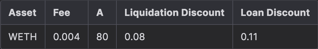
$WETH

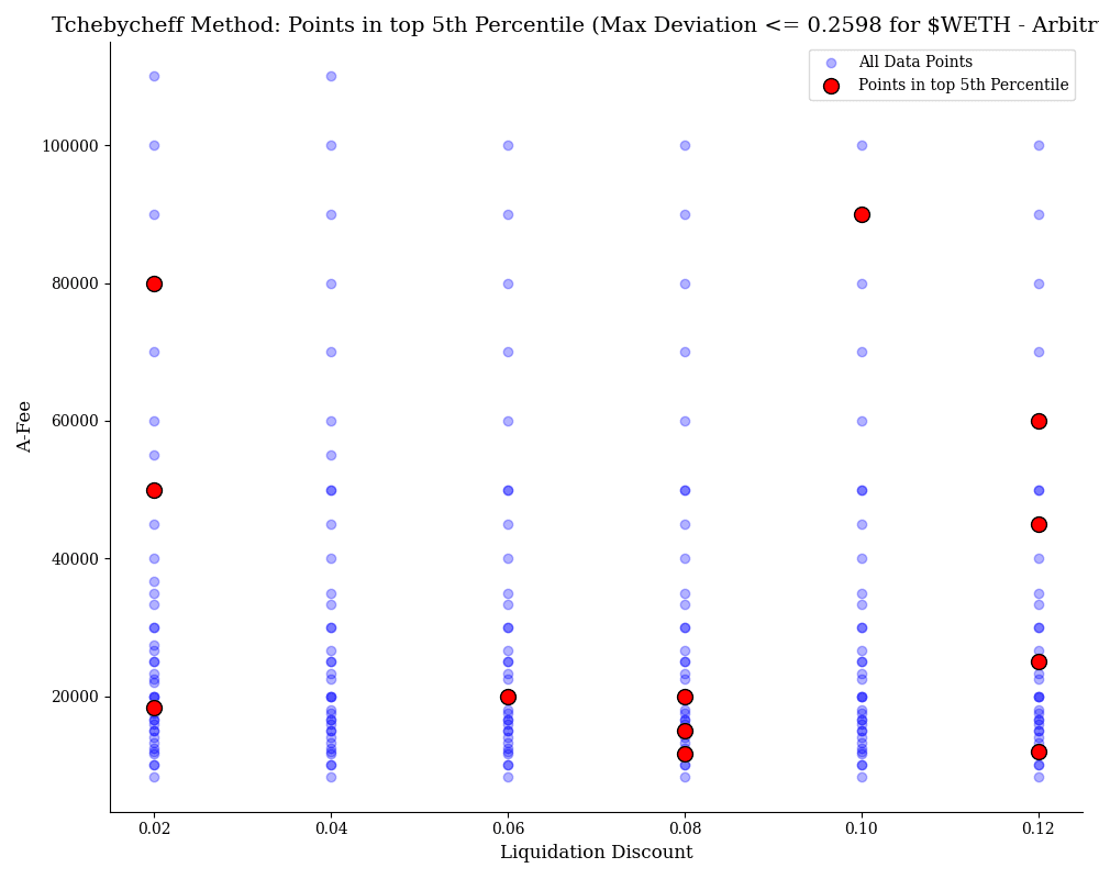
This chart applies the Tchebycheff method to optimize for $WETH on the Arbitrum network by considering multiple constraints, including maximizing Net Llamma Profit Percentage Median, while minimizing Soft Liquidation Loss Percentage Median, Borrower Loss Percentage Median, and Worst Oracle Error Percentage Median. The blue points represent data that did not incur bad debt, showing different combinations of Liquidation Discount and A-Fee (ratio amplification factor and fee). The red points indicate the top 5th percentile of optimal configurations, which balance these constraints according to the Tchebycheff method, with a maximum deviation of 0.2598. These optimal points highlight the best trade-offs between liquidation discount and A-Fee while satisfying the multi-constraint optimization.

After evaluating the valid scenario based on the Techbycheff deviation score and Profitability, we selected the following parameter set:

$wstETH

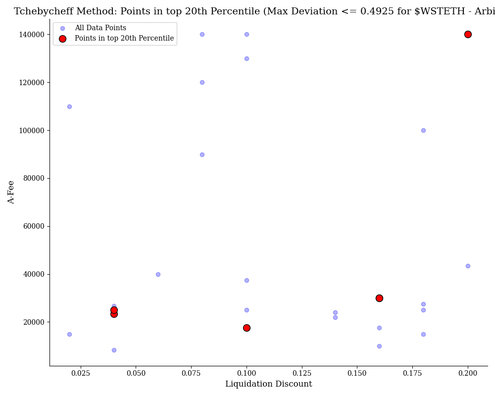
This chart applies the Tchebycheff method to optimize $wstETH on the Arbitrum network, showing the top 20th percentile of data points. The blue points represent combinations of Liquidation Discount and A-Fee (ratio amplification factor and fee) that did not incur bad debt, while the red points highlight the optimal configurations. The red points indicate the best trade-offs, with a maximum deviation of 0.4925.

$WBTC

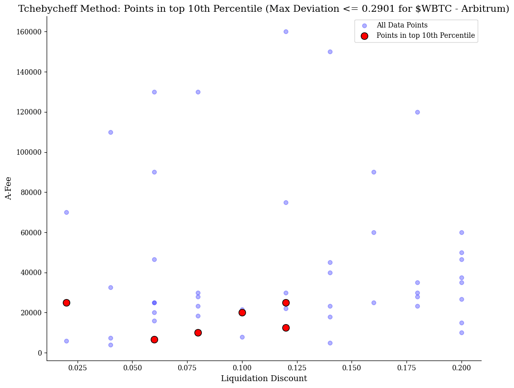
This chart shows the Tchebycheff method's optimization for $WBTC on the Arbitrum network, highlighting points in the top 10th percentile. The blue points represent various Liquidation Discount and A-Fee (ratio amplification factor and fee) combinations that did not incur bad debt, while the red points mark the optimal configurations. The red points reflect the best trade-offs, with a maximum deviation of 0.1807.

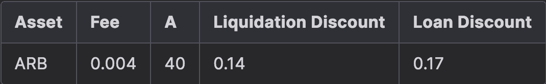
$ARB

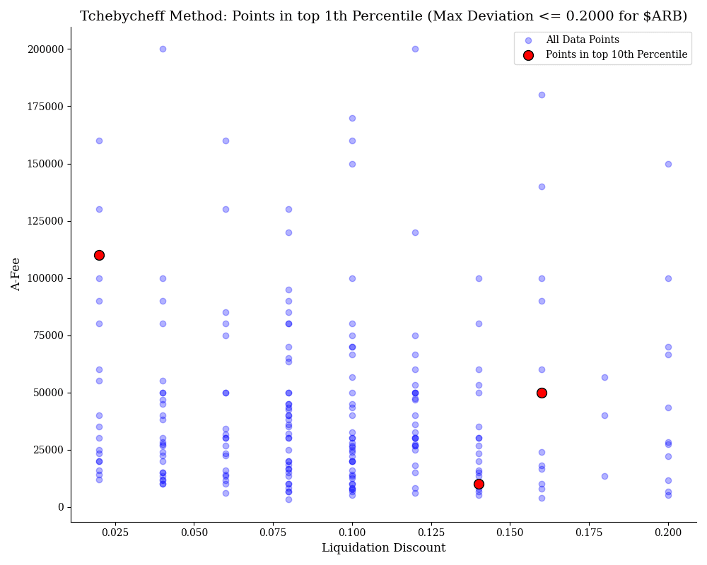
This chart uses the Tchebycheff method to optimize $ARB on the Arbitrum network, focusing on the top 1st percentile of data points. The blue points represent configurations of Liquidation Discount and A-Fee (ratio amplification factor and fee) that did not incur bad debt, while the red points indicate the most optimal combinations. The red points represent the best trade-offs, with a maximum deviation of 0.2000.

$GMX

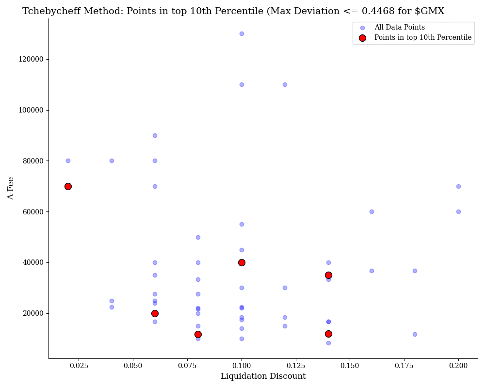
This chart applies the Tchebycheff method to optimize $GMX on the Arbitrum network, showing points in the top 10th percentile. The blue points represent combinations of Liquidation Discount and A-Fee (ratio amplification factor and fee) that did not incur bad debt, while the red points mark the optimal combinations. The optimization maximizes Net Llamma Profit Percentage Median and minimizes Soft Liquidation Loss Percentage Median, Borrower Loss Percentage Median, and Worst Oracle Error Percentage Median. The red points indicate the best trade-offs, with a maximum deviation of 0.4468.

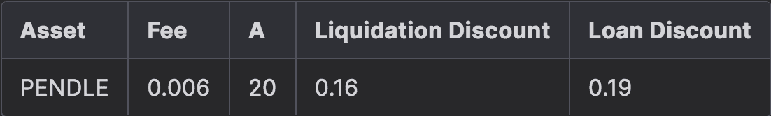
$PENDLE

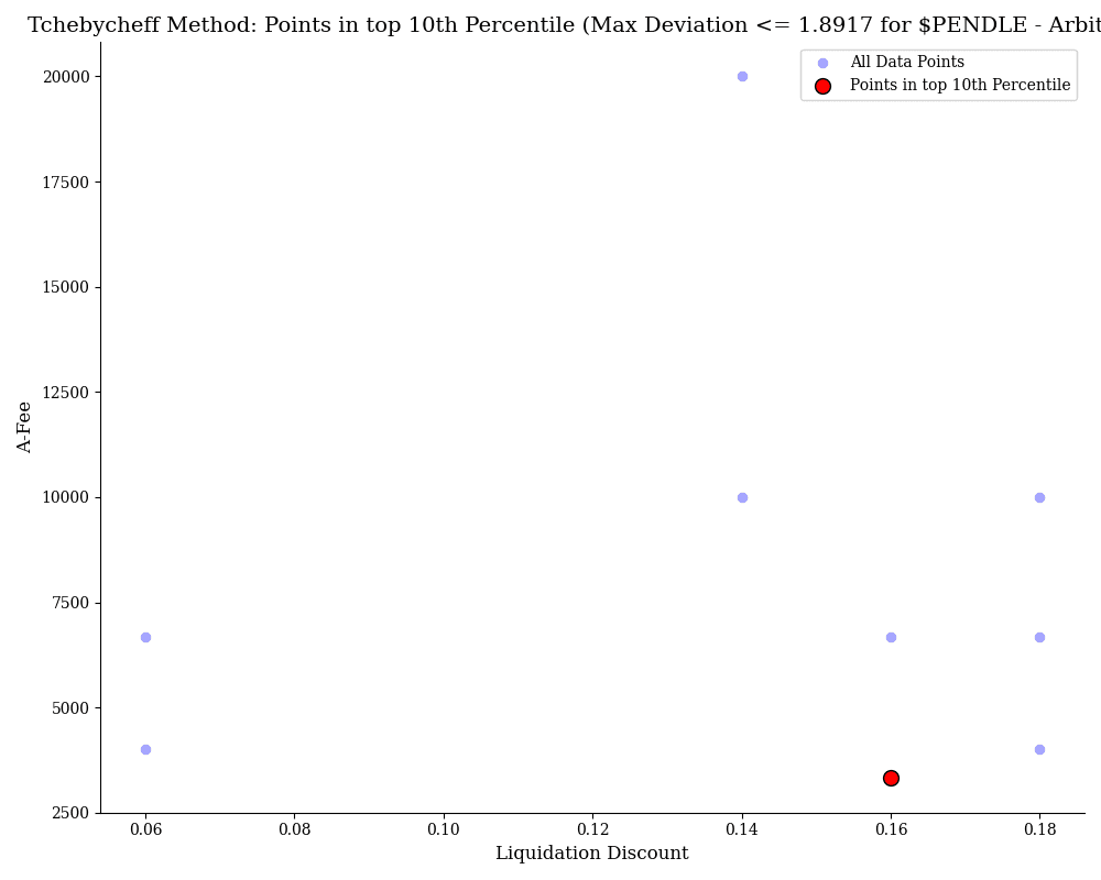
This chart, optimizing $PENDLE on the Arbitrum network using the Tchebycheff method, highlights points in the top 10th percentile. Compared to the other charts, the deviation is significantly higher, at 1.8917, indicating that the trade-offs between the optimization constraints are less optimal. Additionally, there are noticeably fewer viable solutions (red points) in this dataset, suggesting a more limited range of configurations that meet the optimization criteria while maintaining favorable conditions for Liquidation Discount and A-Fee (ratio amplification factor and fee).

$RDNT

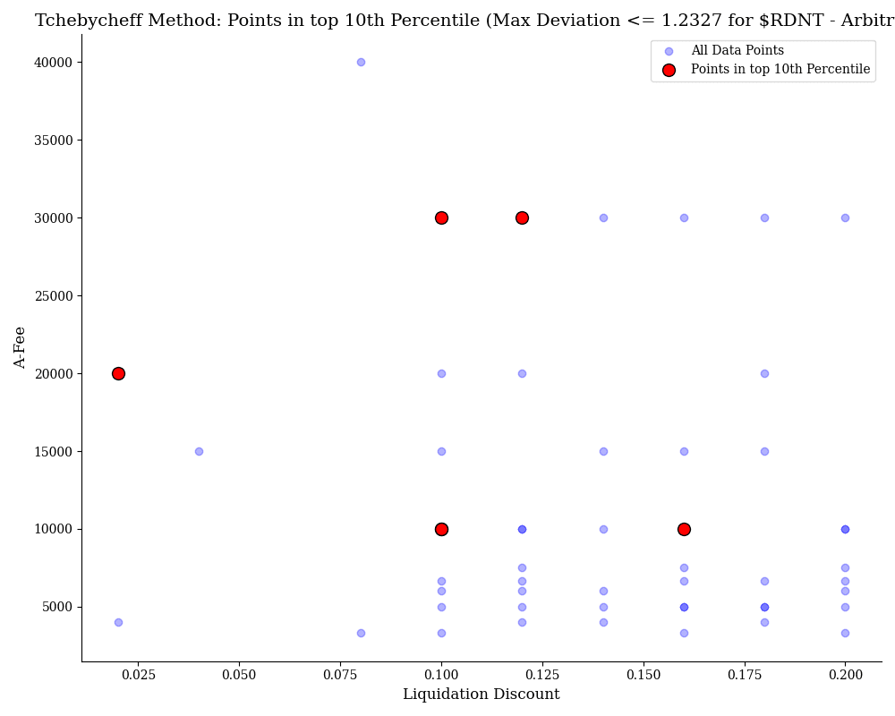
In this chart, the Tchebycheff method optimizes $RDNT on the Arbitrum network, highlighting points in the top 10th percentile. The deviation is relatively high at 1.2327, indicating a less precise optimization compared to other assets. While there are more viable solutions (red points) than in the previous chart, the higher deviation suggests that the trade-offs between the optimization constraints are not as optimal. Despite this, several favorable configurations of Liquidation Discount and A-Fee (ratio amplification factor and fee) are found, primarily concentrated around specific A-Fee values.

4.1.2 Optimism

Below we show the final Techbycheff solutions for assets on Optimism:

$WETH

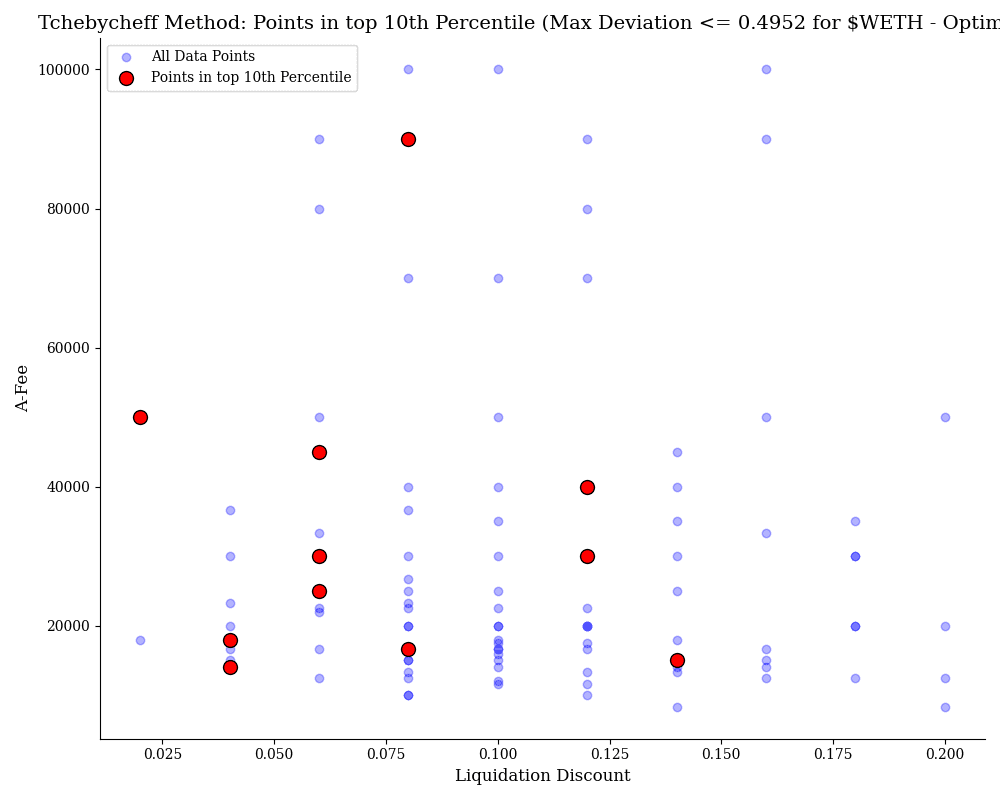
This chart visualizes the Tchebycheff method's optimization for $WETH on the Optimism network, focusing on the top 10th percentile of data points. The maximum deviation, at 0.4952, is moderate, suggesting a decent level of optimization for this dataset. This indicates a wider range of viable solutions compared to other assets, with several optimal points offering favorable trade-offs between risk and reward. The balance between data points and deviation reflects a relatively solid optimization outcome.

$wstETH

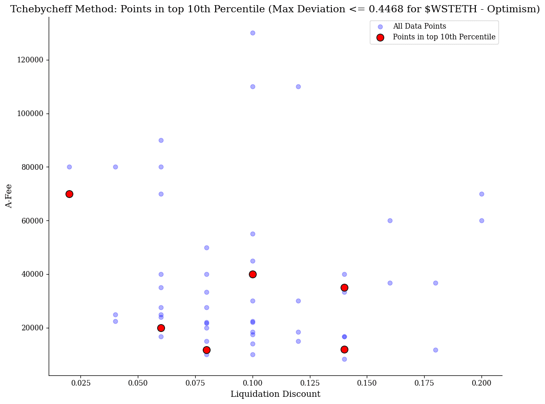
This chart visualizes the Tchebycheff method's optimization for $wstETH on the Optimism network, highlighting points in the top 10th percentile. With a maximum deviation of 0.4468, the optimization is relatively efficient, yielding a moderate number of optimal configurations. The red points represent the most favorable combinations of Liquidation Discount and A-Fee (ratio amplification factor and fee), while the blue points reflect all data points that did not incur bad debt. The red points are scattered across different liquidation discount values, showing a range of viable solutions for optimizing performance under the constraints, with a decent balance between risk and reward.

$WBTC

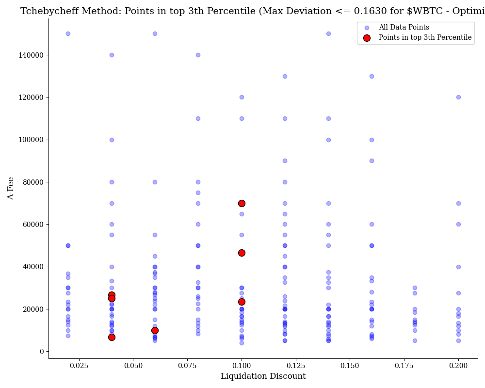
This chart shows the Tchebycheff method's optimization for $WBTC on the Optimism network, highlighting points in the top 3rd percentile. With a relatively low maximum deviation of 0.1630, the optimization is efficient, indicating precise results with several favorable configurations. The red points represent the optimal combinations of Liquidation Discount and A-Fee (ratio amplification factor and fee), while the blue points show all data points that did not incur bad debt. The red points are concentrated around certain liquidation discount values, indicating a narrower but more refined set of viable solutions for optimizing performance within the given constraints.

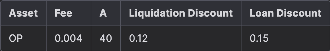
$OP

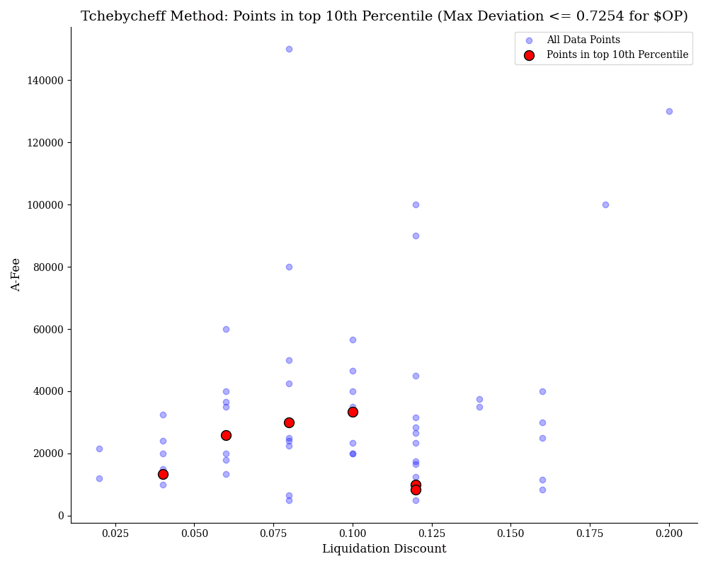
This chart visualizes the Tchebycheff method's optimization for $OP on the Optimism network, highlighting points in the top 10th percentile. With a higher maximum deviation of 0.7254, the optimization is less precise compared to other assets, suggesting a wider range of trade-offs. The red points, representing the most optimal configurations of Liquidation Discount and A-Fee (ratio amplification factor and fee), are spread across different liquidation discount values, reflecting a diverse set of possible solutions. The blue points show all data points that did not incur bad debt. Despite the higher deviation, several configurations still offer favorable trade-offs, although the optimization may allow for more variability in the outcomes.

The recommended parameter set is:

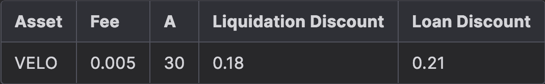
$VELO

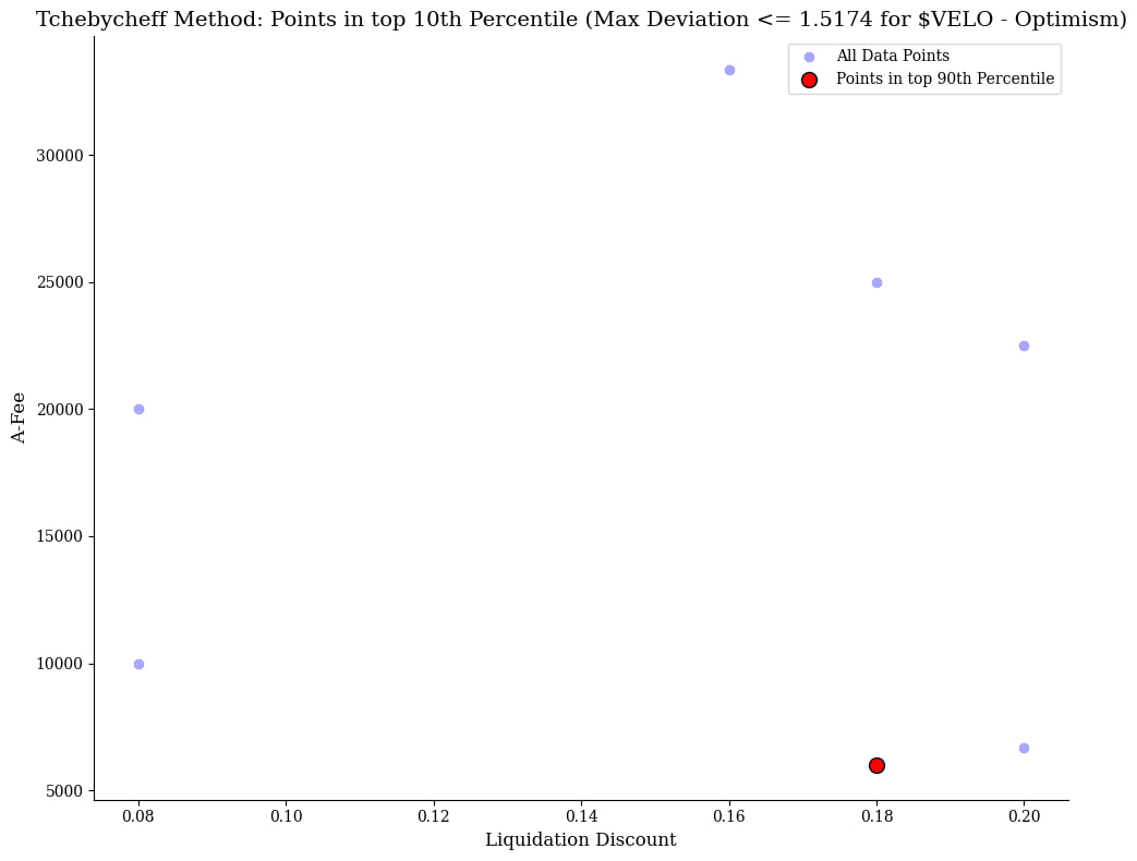
This chart shows the Tchebycheff method's optimization for $VELO on the Optimism network, focusing on points in the top 10th percentile. The maximum deviation is quite high at 1.2573, indicating a less precise optimization and a wider range of acceptable trade-offs. The red points represent the optimal combinations of Liquidation Discount and A-Fee (ratio amplification factor and fee), with very few viable solutions identified. The blue points represent all data points that did not incur bad debt, but the sparse distribution of optimal (red) points suggests limited opportunities for optimal configurations under the given constraints. This higher deviation and the lack of multiple viable solutions point to greater difficulty in finding ideal trade-offs for $VELO.

The recommended parameter set is:

4.2 Debt Ceiling

We identified the kink of liquidity for each chain collateral asset for collateral swaps into USDC/USDT. The results are displayed below per chain and the debt ceiling is marked for the respective asset in terms of the collateral asset. For this we fetched quotes periodically from Kyberswap and Paraswap between 2024-08-04 to 2024-08-13.

Note: USDC pairs tend to have a higher liquidity profile compared to USDT, which seems to be due to more extensive DeFi integrations and DEX pairings. The methodology here can be expanded upon with an aggregated model across all major stablecoins in a chain.

4.2.1 Arbitrum

$WETH

This chart displays the price impact of swapping $WETH into USDC/USDT. The debt ceiling is set at 4,848.30 WETH, beyond which price impact escalates significantly, indicating higher slippage for swaps above this amount.

$WBTC

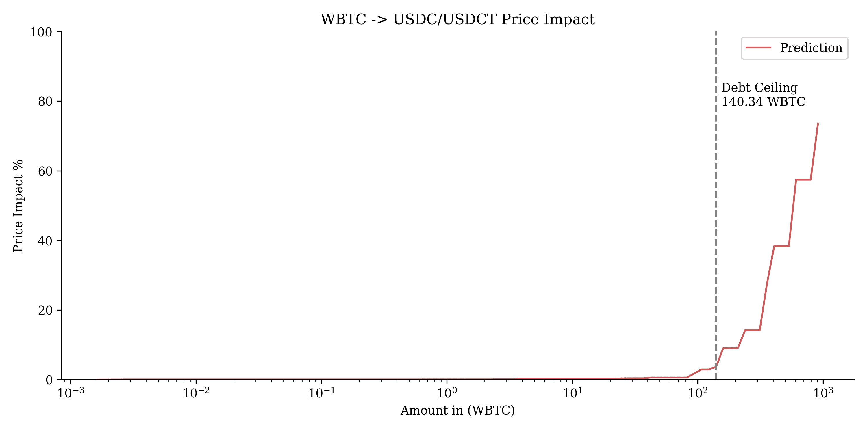
This chart shows the price impact of swapping $WBTC into USDC/USDT. The debt ceiling is set at 140.34 WBTC, beyond which price impact increases rapidly, indicating higher slippage for larger swaps above this threshold.

$WSTETH

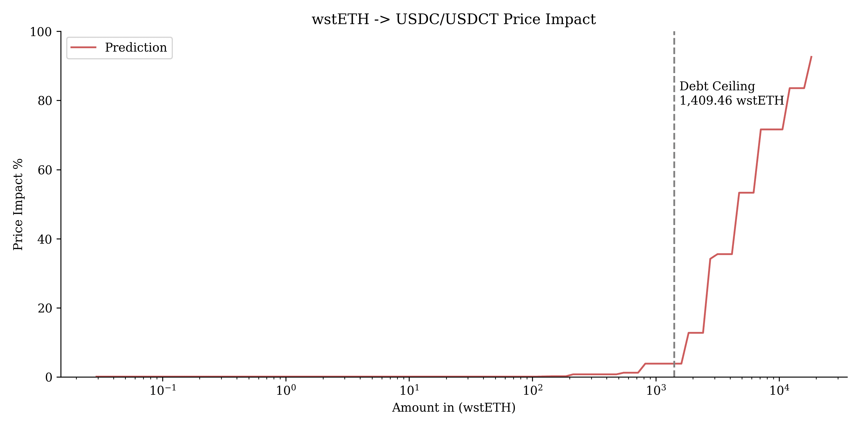
This chart shows the price impact of swapping $wstETH into USDC/USDT. The debt ceiling is set at 1,409.46 wstETH, beyond which the price impact rises sharply, indicating significant slippage for swaps exceeding this amount.

$ARB

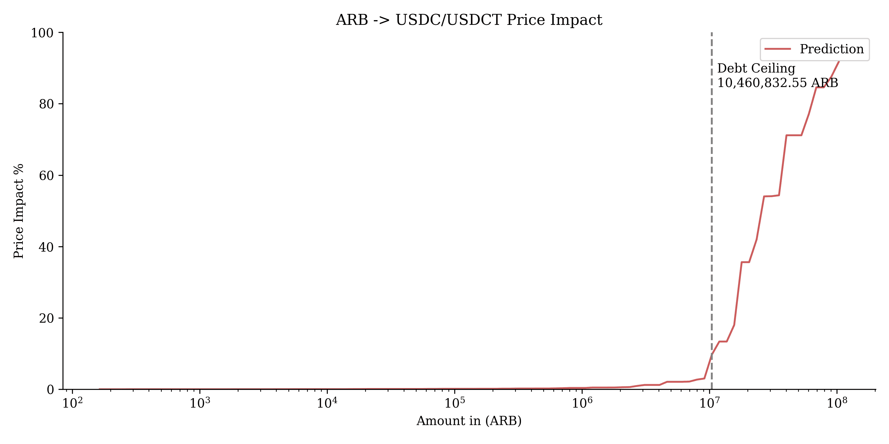
This chart shows the price impact of swapping $ARB into USDC/USDT as a function of the amount of $ARB swapped. The x-axis represents the amount of $ARB in logarithmic scale, while the y-axis indicates the corresponding price impact percentage. A sharp rise in price impact occurs beyond the debt ceiling of 10,460,832.55 ARB, marked by the vertical dashed line. This demonstrates the liquidity limit for $ARB collateral swaps, where any amounts exceeding this threshold result in significant price slippage, making larger swaps much more costly.

$GMX

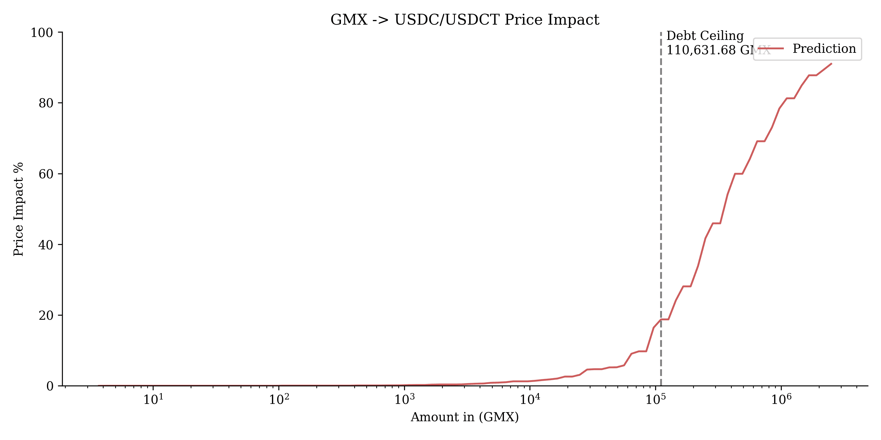
This chart shows the price impact of swapping $GMX into USDC/USDT. The x-axis represents the amount of $GMX swapped, while the y-axis shows the percentage of price impact. Beyond the debt ceiling of 110,631.68 GMX, marked by the vertical dashed line, price impact increases significantly, indicating a sharp rise in cost for larger swaps beyond this threshold.

$PENDLE

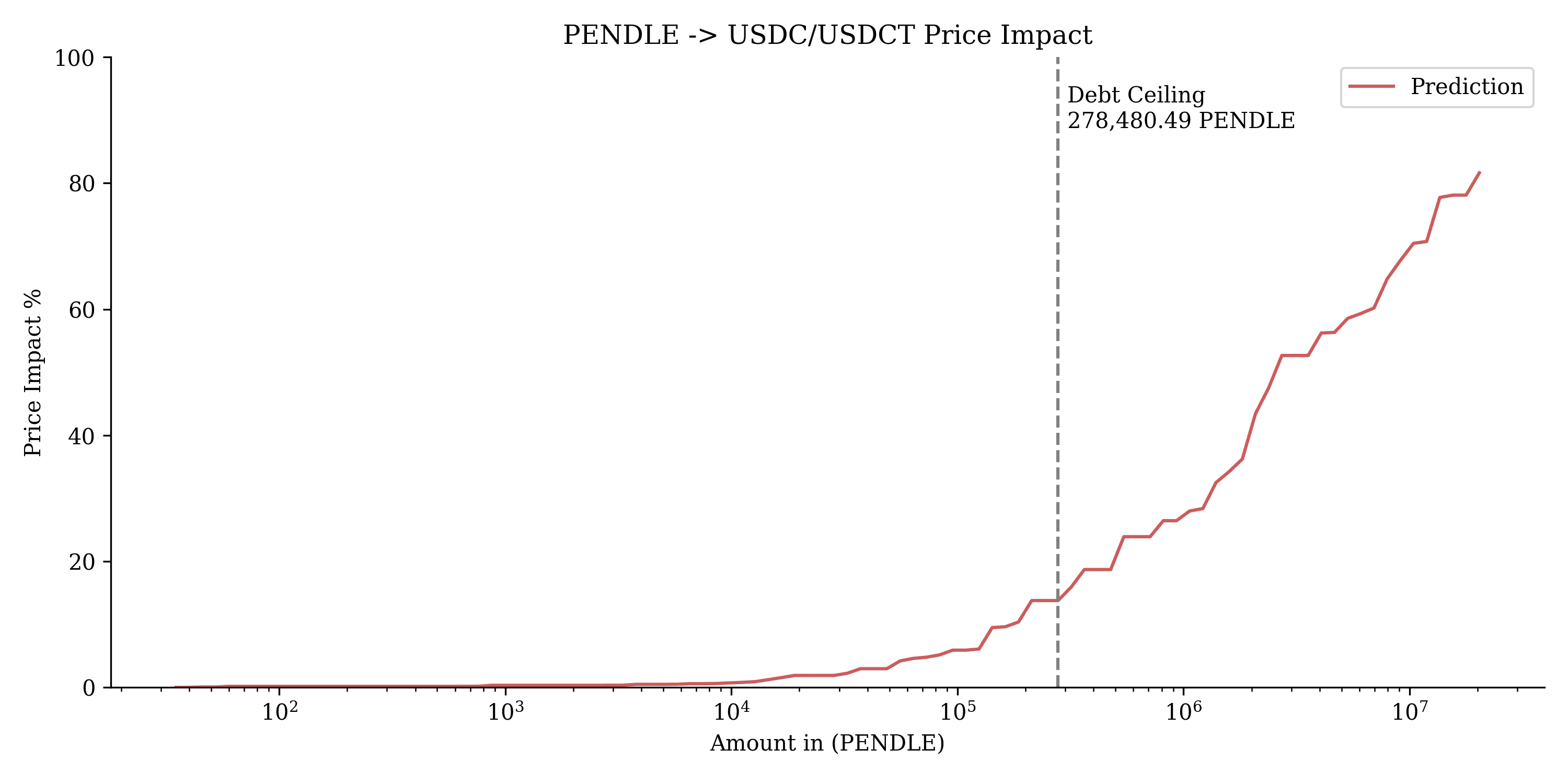
This chart shows the price impact of swapping $PENDLE into USDC/USDT. The debt ceiling is marked at 278,480.49 PENDLE, beyond which price impact increases significantly, leading to greater slippage for larger swaps.

$RDNT

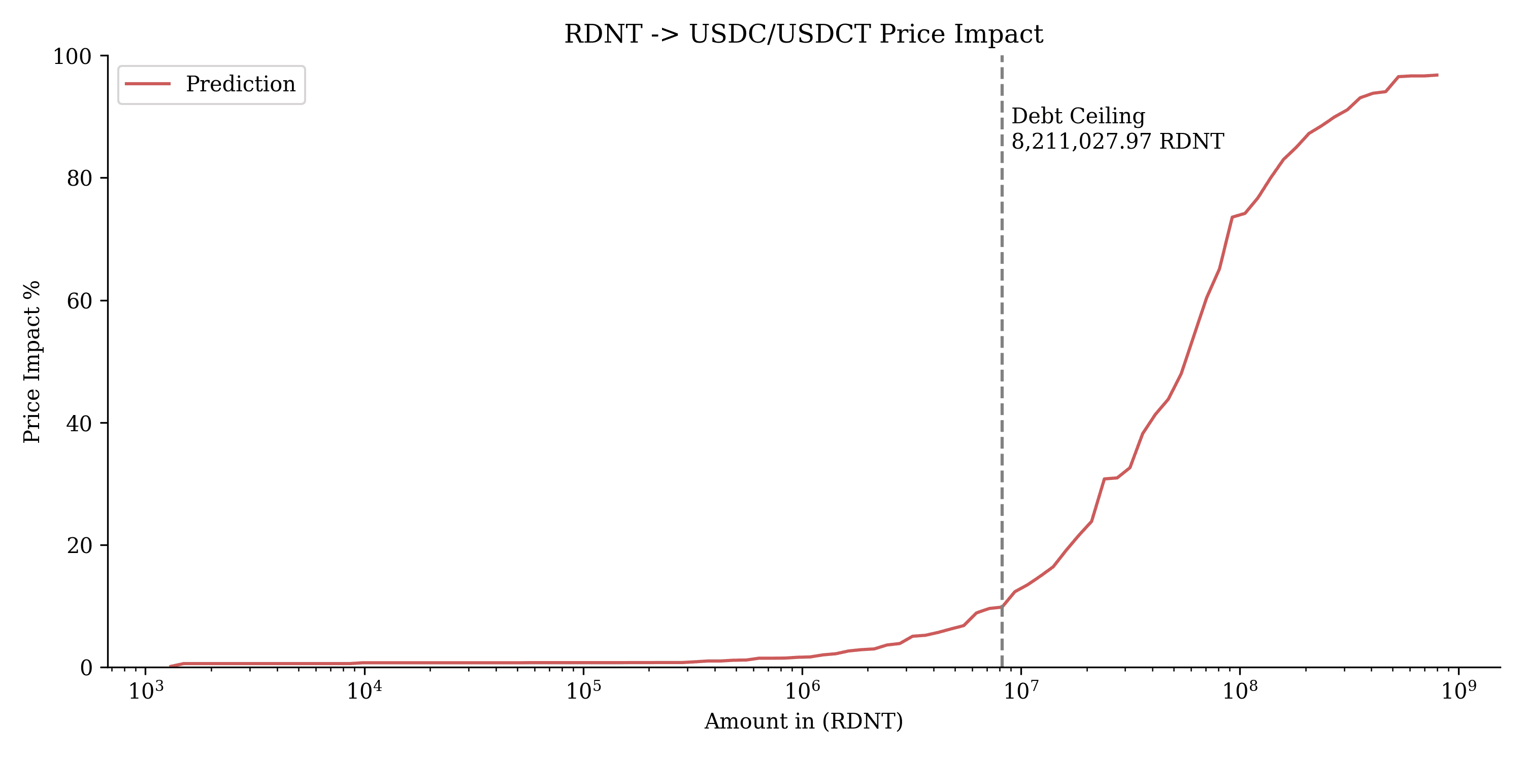
This chart displays the price impact of swapping $RDNT into USDC/USDT. The debt ceiling is set at 8,211,027.97 RDNT, after which price impact increases steeply, indicating higher slippage for larger swaps beyond this threshold.

4.2.2 Optimism

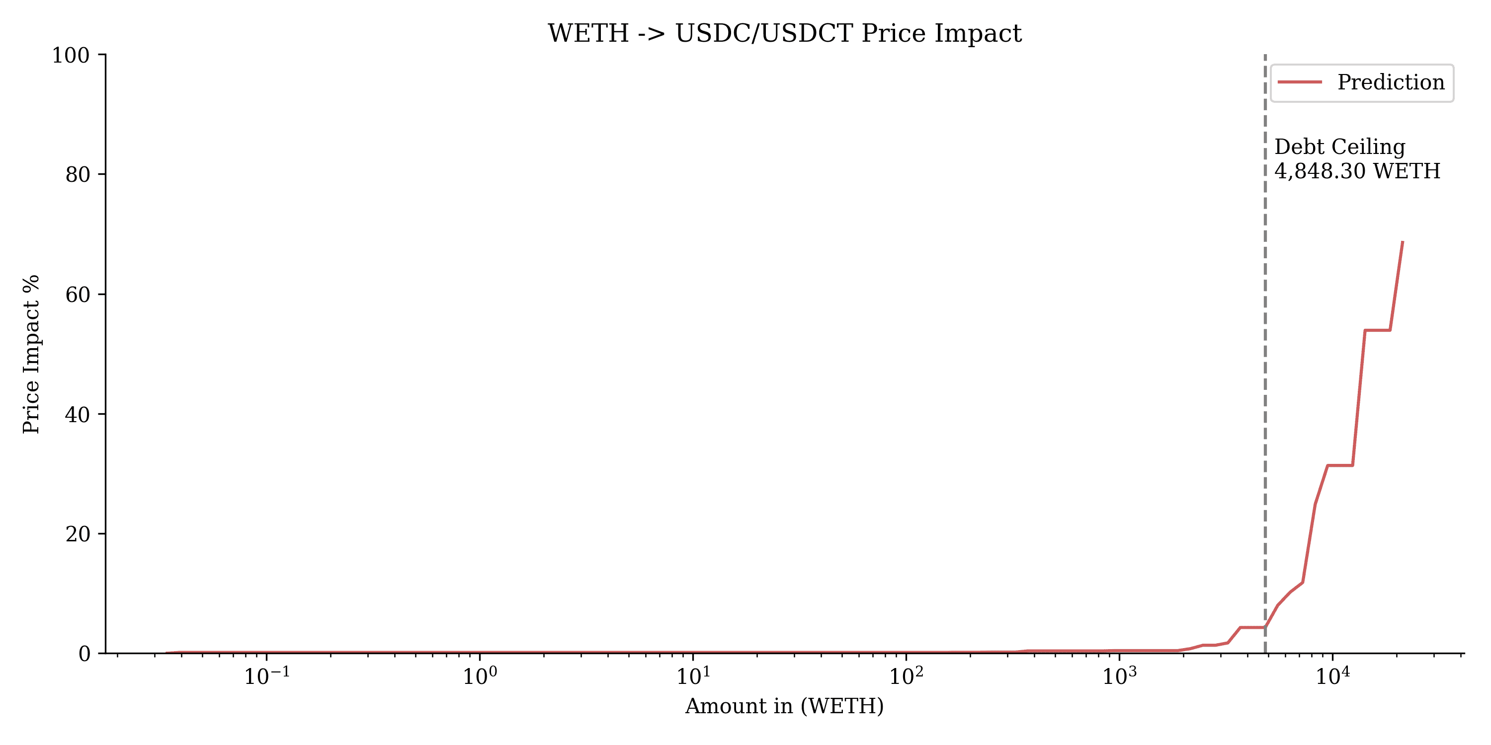
$WETH

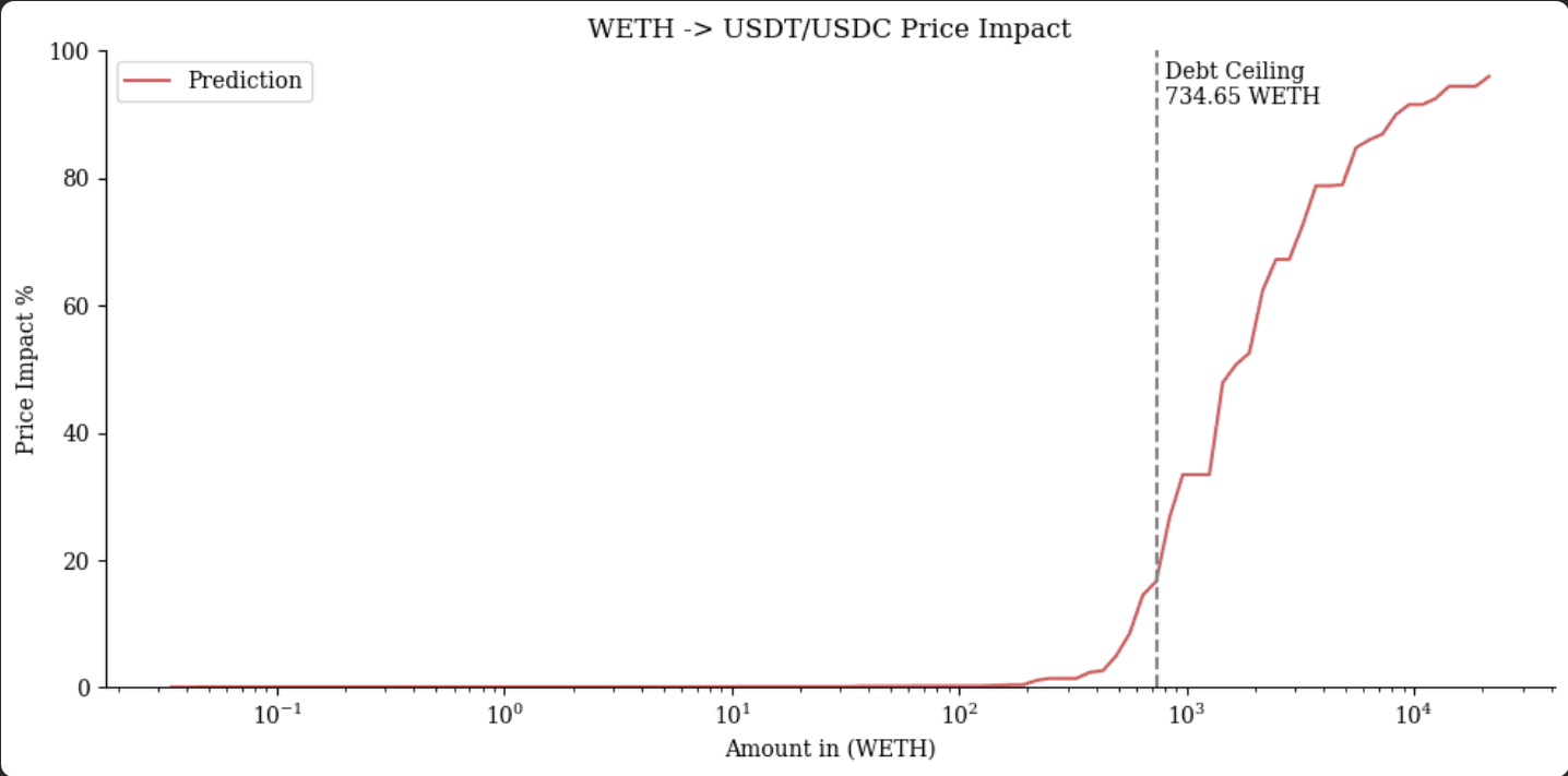
This chart shows the price impact of swapping $WETH into USDC/USDT. The debt ceiling is set at 734.65 WETH, beyond which the price impact increases sharply, indicating larger slippage for swaps exceeding this threshold.

$WBTC

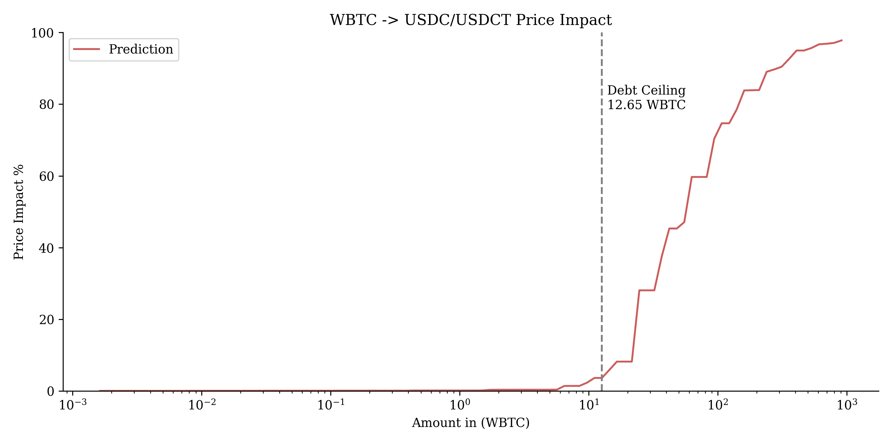
This chart depicts the price impact of swapping $WBTC into USDC/USDT. The debt ceiling is marked at 12.65 WBTC, after which the price impact rises sharply, indicating increased slippage for larger swaps beyond this threshold.

$WSTETH

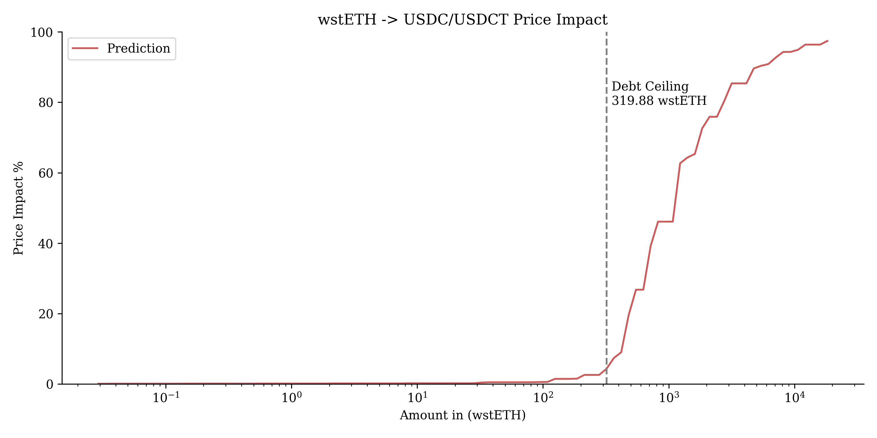
This chart shows the price impact of swapping $wstETH into USDC/USDT. The debt ceiling is set at 319.88 wstETH, beyond which the price impact increases significantly, indicating larger slippage for swaps exceeding this threshold.

$OP

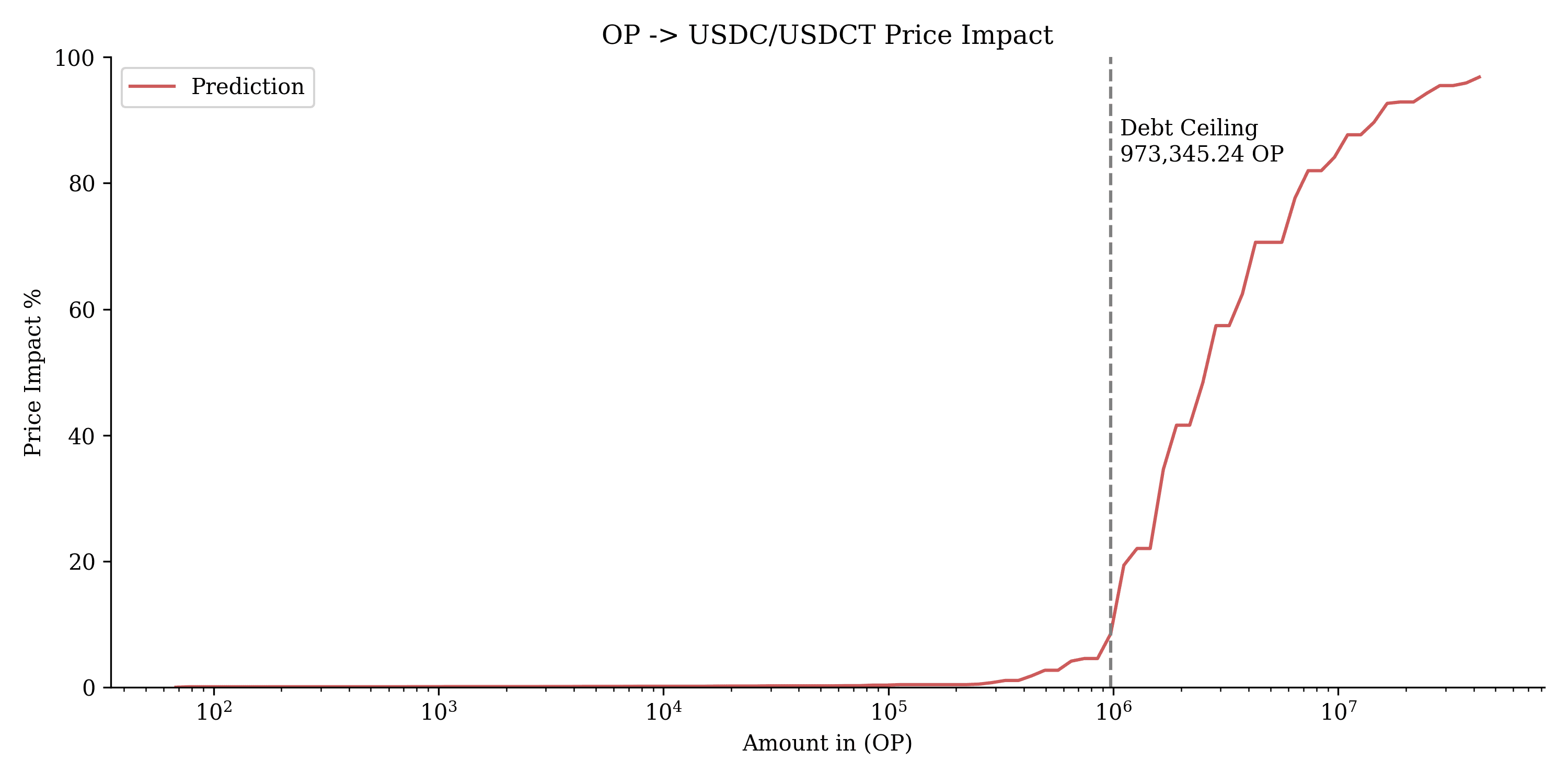
This chart illustrates the price impact of swapping $OP into USDC/USDT. The vertical dashed line marks the debt ceiling of 973,345.24 OP, beyond which price impact rises sharply, indicating increased slippage for larger swaps.

$VELO

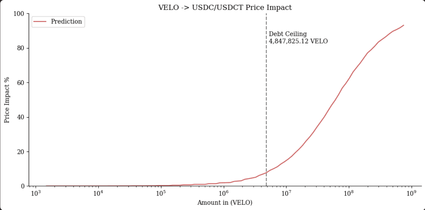
This chart illustrates the price impact of swapping $VELO into USDC/USDT. The debt ceiling is marked at 4,847,825.12 VELO, beyond which the price impact increases steadily, showing significant slippage for larger swaps above this threshold.

Section 5: Recommendations

After analyzing the simulation results across various assets on Arbitrum and Optimism, we provide tailored recommendations for each asset based on performance, price impact, and market liquidity, along with the suggested debt ceilings.

The following assets have met suitable criteria for onboarding with optimal parameters based on our simulation provided. Some of these markets have already been onboarded with our initial parameter recommendations. The individual reviews below outline the comparison to initial recommendations, and we do not consider it necessary to make immediate changes to existing markets at this time.

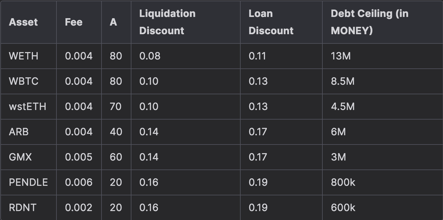
Recommended parameterization for collateral tokens on Arbitrum

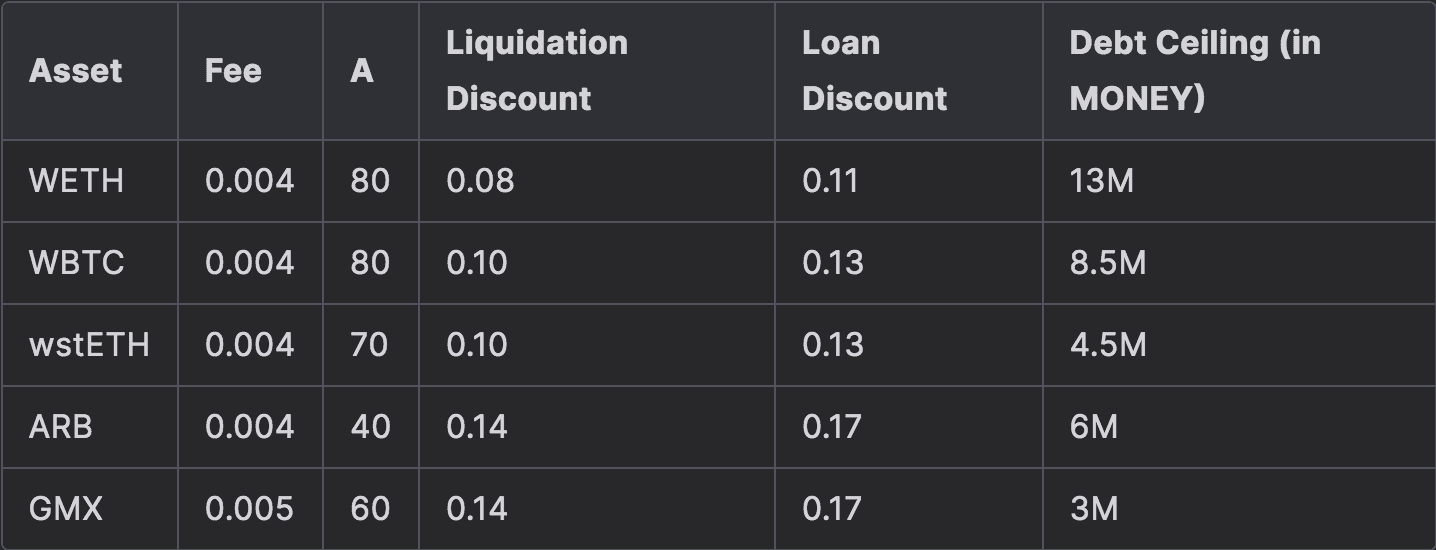
Recommended parameterization for collateral tokens on Optimism

5.1 Recommendations for Arbitrum

5.1.1 WETH

Based on our simulations, $WETH performed consistently well with a balanced trade-off between liquidation discount and A-Fee. The results show minimal bad debt scenarios and the Tchebycheff method yielded stable optimal configurations. The liquidity curve further suggests that $WETH can handle larger swaps without significant slippage. The debt ceiling of 4,848.30 WETH (13M MONEY) is recommended to avoid price impact spikes.

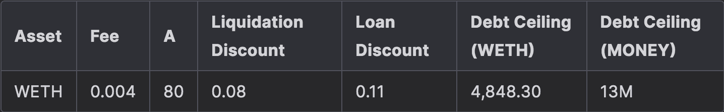
Recommendation: We recommend maintaining the current parameters for the existing $WETH market on Arbitrum, noting that the market has been instantiated with our initially recommended values of fee: 0.2%, A: 72, liquidation_discount: 4%, loan_discount: 7%. The current debt ceiling of the $WETH-Arbitrum market is 1.5M MONEY. From a market risk perspective, it can be safely raised to 13M max debt.

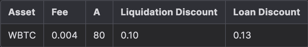
5.1.2 WBTC

For $WBTC, the simulations output suggested minimal deviations in Tchbycheff method. A debt ceiling of 140.34 WBTC (8.5M MONEY) is recommended to manage slippage effectively.

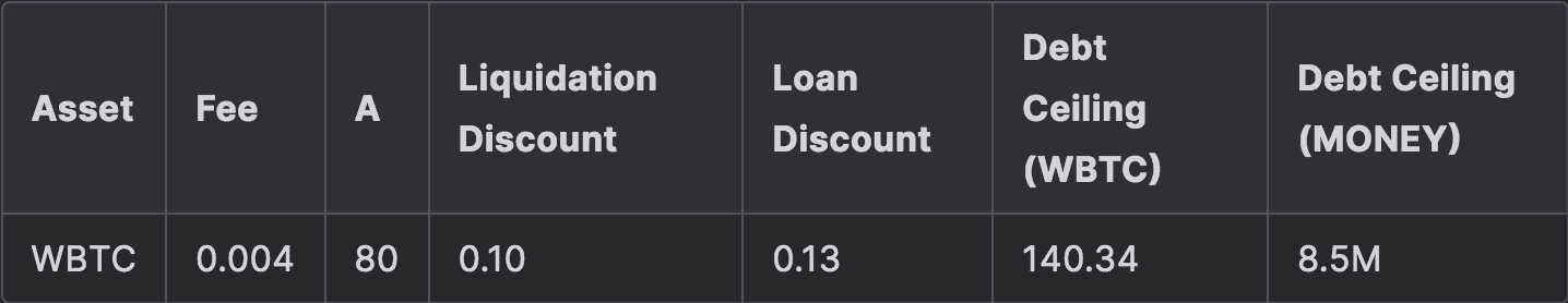
Recommendation: We recommend maintaining the current settings for the existing $WBTC-Arbitrum market, noting that it has been instantiated with our initial recommended values of fee: 0.2%, A: 89, liquidation_discount: 4%, loan_discount: 7%. The current debt ceiling of the $WBTC-Arbitrum market is 800K MONEY. From a market risk perspective, it can be safely raised to 8.5M max debt.

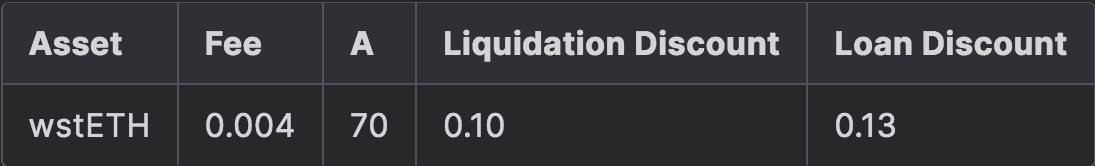
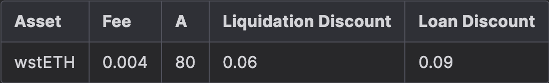
5.1.3 wstETH

$wstETH similarly produced stable results with minimal bad debt across the scenarios tested. The top 20th percentile configuration offers a good balance between risk and profit, supported by a recommended debt ceiling of 1,409.46 wstETH (4.5M MONEY).

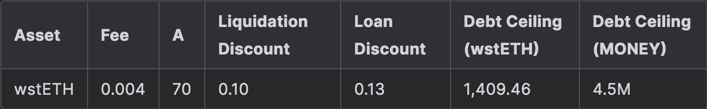
Recommendation: We recommend onboarding $wstETH with the parameters and debt ceiling provided.

5.1.4 ARB

$ARB demonstrated a strong performance in our analysis, with favorable results across all constraints. The optimization process yielded a robust configuration with limited deviations, and the liquidity curve indicates that $ARB can accommodate sizable swaps before encountering steep slippage. A debt ceiling of 10,460,832.55 ARB is recommended to balance liquidity and price impact.

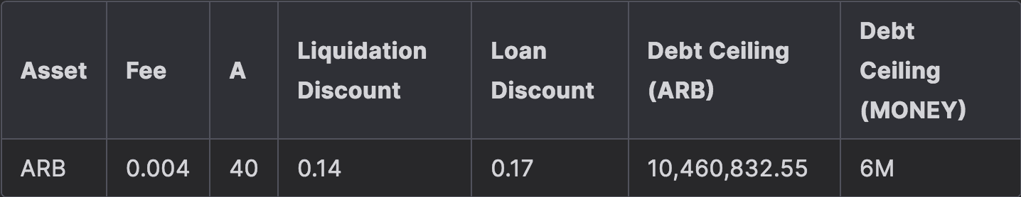
Recommendation: We recommend maintaining the current parameter configuration for the $ARB market, noting that it has been instantiated with our initial recommendations of fee: 0.15%, A: 30, liquidation_discount: 9%, loan_discount: 12%. The current debt ceiling of the $ARB market is 200K MONEY. From a market risk perspective, it can be safely raised to 6M max debt.

5.1.5 GMX

$GMX performed reliably, with well-distributed optimal points in the top 10th percentile of configurations. Liquidity analysis indicates that $GMX can manage moderately large swaps without significant slippage. A debt ceiling of 110,631.68 GMX (3M MONEY) is recommended to avoid excess price impact.

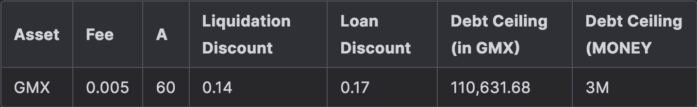
Recommendation: We recommend onboarding $GMX with the parameters and debt ceiling provided.

5.1.6 PENDLE

$PENDLE's performance, though adequate in some cases, showed high deviation in optimization outcomes, indicating limited viable solutions. Liquidity curves are thin, with a debt ceiling of 278,480.49 PENDLE (800K MONEY) indicating that the market may not support large swaps without significant slippage. Given these concerns, we advise against continuing with $PENDLE.

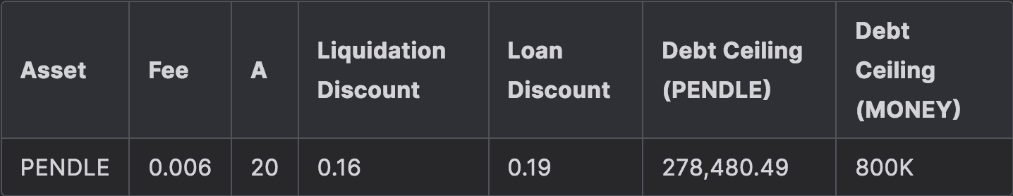
Recommendation: We do not recommend onboarding $PENDLE due to volatility and thin liquidity.

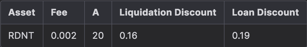
5.1.7 RDNT

$RDNT presented similar issues to $PENDLE, with high deviation and limited optimal configurations. The liquidity profile is too thin, with a debt ceiling of 8,211,027.97 RDNT (600K MONEY) leading to significant slippage even with moderate swaps. This poses a risk of volatility.

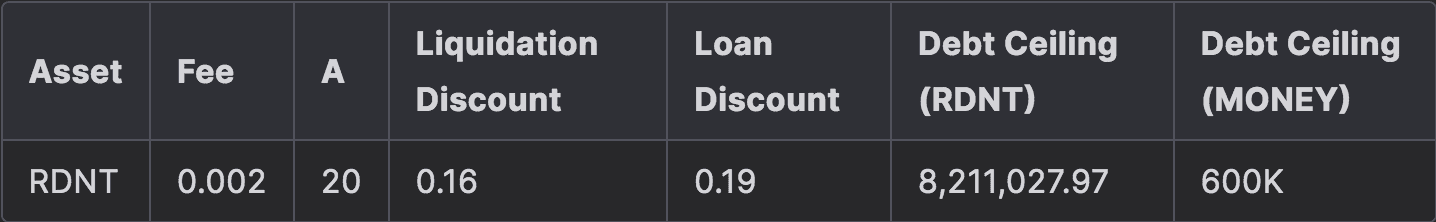
Recommendation: We do not recommend onboarding $RDNT due to the volatility and thin liquidity.

5.2 Recommendations for Optimism

5.2.1 WETH

$WETH on Optimism showed consistent performance with a moderate maximum deviation, resulting in stable configurations in the top 10th percentile. Liquidity analysis indicates $WETH can manage a healthy amount of swaps with acceptable slippage. A debt ceiling of 490.32 WETH (1.1M MONEY) is recommended to avoid excessive price impact.

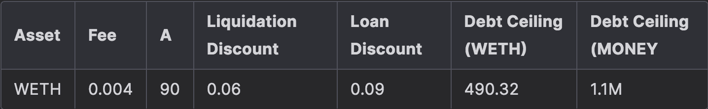
Recommendation: We recommend continuing with the current parameter configuration for the $WETH market, noting that it has been instantiated with our initial recommendations of fee: 0.2%, A: 72, liquidation_discount: 4%, loan_discount: 7%. The current debt ceiling of the $WETH market is 1.75M MONEY. As current debt is only ~162K MONEY, we recommend reducing the debt ceiling to 1.1M until further review.

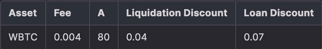
5.2.2 WBTC

$WBTC performed exceptionally well with precise optimization results. The liquidity analysis indicates that it can handle moderate swaps without encountering high slippage, making it a reliable asset on Optimism. A debt ceiling of 12.65 WBTC (800K MONEY) is recommended to maintain a balanced liquidity profile.

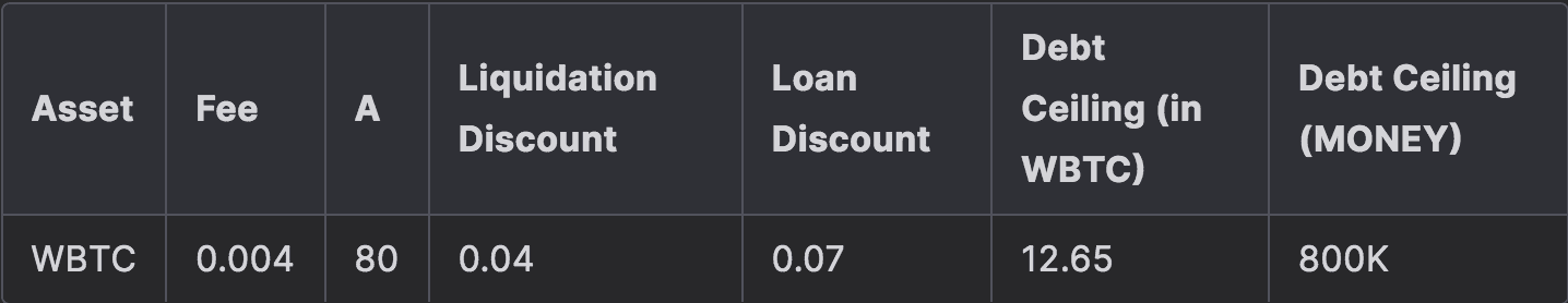
Recommendation: We recommend continuing with the current parameter configuration for the $WBTC market, noting that it has been instantiated with our initial recommendations of fee: 0.2%, A: 89, liquidation_discount: 4%, loan_discount: 7%. The current debt ceiling of the $WBTC market is 250k MONEY. From a market risk perspective, it can be safely raised to 800K max debt.

5.2.3 wstETH

$wstETH on Optimism performed well with a balanced trade-off between risk and reward, supported by adequate liquidity to manage moderately large swaps. The optimization results suggest that it can continue to perform with minimal bad debt risk. A debt ceiling of 319.88 wstETH (1M MONEY) is recommended to keep swaps within manageable price impact.

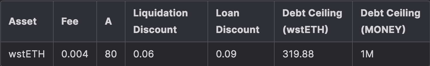
Recommendation: We recommend continuing with the current parameter configuration for the $wstETH market, noting that it has been instantiated with our initial recommendations of fee: 0.2%, A: 72, liquidation_discount: 4%, loan_discount: 7%. The current debt ceiling of the $wstETH market is 500k MONEY. From a market risk perspective, it can be safely raised to 1M max debt.

5.2.4 OP

$OP on Optimism showed slightly more volatility with a higher maximum deviation, but several viable configurations were identified. The liquidity curve supports moderate swaps, though the slippage increases for larger transactions. A debt ceiling of 973,345.24 OP (1.5M MONEY) is recommended to balance liquidity and price impact.

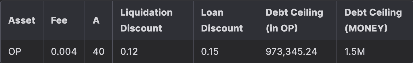
Recommendation: We recommend onboarding $OP with the parameters and debt ceiling provided.

5.2.5 VELO

$VELO demonstrated less precise optimization results, with high deviation and fewer viable solutions. Liquidity is limited, making larger swaps difficult without significant slippage. A debt ceiling of 4,847,825.12 VELO (350K MONEY) is recommended to manage liquidity efficiently, though the results indicate caution.

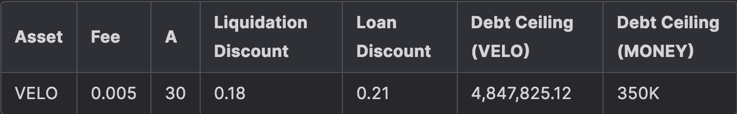
Recommendation: We do not recommend onboarding $VELO due to the volatility and thin liquidity.

Section 6: Future Work

There are opportunities to continue improving the crvUSDrisk sim tool by refining its assumptions and optimizing its performance. There are also additional experiments that can build on the foundation laid by this tool, including optimizing MONEY pool liquidity. This section addresses various areas of research and development that may be additional value adds to the defi.money protocol.

6.1 Exogenous Collateral Price Paths

Limitation: No price impact modeling

Collateral price paths are generated synthetically using mathematical finance tools. No market friction is assumed, meaning that during the liquidation process, the sale of collateral does not cause any price changes. This is a limiting assumption, particularly when the liquidity of the collateral is highly volatile. In scenarios where the debt-to-liquidity ratio of a collateral asset remains stable, effective liquidations can be ensured by setting an appropriate debt ceiling. However, if there is a significant change in the liquidity of the collateral asset, it may be necessary to model the price impact of the collateral sale.

Future Work: Incorporate Price Impact into the Price Trajectories

There are two methods to incorporate price impact into collateral price paths. First, one assumes that the impact will be arbitraged away within the next few blocks. In this scenario, a collateral sale results in a sudden price drop, modeled as a jump, that is subsequently corrected back to the original spot price. Second, one assumes the price impact is temporarily permanent, meaning the collateral price remains affected for a longer duration. Selecting between these two approaches is challenging as it requires an understanding of market-making incentives. However, the second assumption can be modeled by making rough assumptions about the volatility of price paths. Therefore, the first assumption is generally sufficient for modeling price impact.

Value Add: Precise modeling of assets where the debt from the collateral is relatively high compared to its liquidity depth

While the protocol is in an early stage of growth and limits inclusion to collateral types with strong liquidity assurances, modeling price impact of liquidation is not a priority. It may become an essential consideration as the MONEY supply increases and the protocol wishes to consider assets with less market maturity.

6.2 Endogenous Liquidity Dynamics

Limitation: Model does not account for black swan events

When creating a simulation run, the liquidity of the assets involved evolves solely through the trades of arbitrageurs and liquidators. This assumption applies to all scenarios except those involving drastic liquidity changes due to external factors. The objective is to assess the system's resilience to exponential decreases in liquidity and to evaluate how quickly liquidators can repay the debt before it becomes unprofitable to do so.

Future Work: Additional liquidity experiments

The current simulator models static low liquidity scenarios. An additional experiment that would be valuable to model involves addressing the following question: In the event of an exponential decrease in liquidity, can liquidators repay the debt of liquidation-eligible positions quickly enough to prevent them from becoming undercollateralized?

Value Add: Enhance emergency preparedness

It may be valuable to have advance insight into black swan scenarios such as may periodically occur in assets with high venue concentration, usually associated with poor market maturity or adoption. External factors that may dramatically change the liquidity profile of the asset can affect the solvency of defi.money, and accurately modeling the potential severity and protocol resiliency of such scenarios can help to avoid unsuitable exposures to high-risk assets.

6.3 Simulator Code Optimization

Limitation: Simulation runs are very time-consuming

Dependencies of the simulation tool use external Python implementations of crvUSD smart contracts. These implementations are a direct transposition from Vyper language to Python. Hence unnecessary inefficiencies, like fixed point calculations, limit the speed of execution.

Future Work: Code Optimizations

The simulation heavily uses 0xreview's crvusdsim for simulating the protocol. Since the code for that is slightly modified Vyper code to make it run in Python, it would be very beneficial in the long run to make it more optimized. Some of the potential optimizations could be:

• Reduce uint256 <-> float conversions and make the whole codebase strictly follow float for optimizations

• Remove for loops to numpy array operations to save time (and if possible we can use JIT compilation using Numba)

• Modify Vyper math functions to numpy functions (for example log2)

Value Add: Allow enhanced protocol health monitoring

At the early stage of the protocol, when it has only onboarded a handful of assets, simulation run optimization is not a priority. It may be desirable to have access to semi-regular simulation updates that assess, for example, dynamic shifts in collateral liquidity and/or MONEY supply. Such runs would naturally be accessible from the defi.money Risk Portal, giving more nuanced insight into the health of the protocol, and informing the need for changes like debt ceiling adjustments. As the protocol expands across chains and collateral types, it will become increasingly important to further improve optimizations.

6.4 MONEY Liquidity Optimization

Limitation: Minimum MONEY liquidity provision requirements are not precisely known

Although it is known that available MONEY liquidity is essential to properly facilitate liquidations, the precise requirements are unclear. The simulation tool establishes a foundation to test the system under different conditions, although experimentation in this regard would require the development of additional methodologies.

Future Work: Pegkeeper modeling and liquidity experimentation

The expanded model would incorporate the global market for the MONEY token and precisely model arbitrage between the Pegkeeper pools. This requires an assessment of the performance of the Pegkeepers under various conditions and with scaled levels of overall liquidity. Testing various liquidity levels during adverse market scenarios allows us to observe variations in bad debt accrual from missed liquidations.

Value Add: Improved resource allocation

Having precise insight into MONEY liquidity requirements at a given time can help stakeholders more efficiently allocate resources. Liquidity provision is likely to be financed through gauge emissions, which requires stakeholders to have either a financial motive or protocol health motive to gauge vote. Recommendations based on simulation output may align stakeholders to ensure adequate liquidity provision and have the confidence that their resources are allocated optimally.