Introduction

This document first presents a general methodology that LlamaRisk uses to craft protocol-specific or market-specific supply cap and borrow cap recommendations. Secondly, we explain our modified methodology for use with crvUSD and LlamaLend, which have the unique property of soft liquidations facilitated through arbitrage.

Caps are placed to ensure lenders can exit when needed and with their principal amount in the least case. In other words, with proper cap recommendations, we ensure there is no possibility of bad debt in the market under observation.

We determine a cap by modeling a hypothetical adverse scenario (price shock) in which, based on the current user behavior, the liquidatable collateral and the liquidatable debt do not result in negative liquidator profit. Those caps will be our most aggressive quotes for acceptable protocol exposure. Furthermore, we can assign a recommended cap that maximizes expected liquidator profit, meaning the available liquidity is sufficient to accommodate liquidation events with minimal price impact.

General Methodology

The general debt ceiling methodology described here is the foundation we use to determine suitable exposure limits for all lending markets. The subsequent section will address protocol-specific considerations that require modification of this methodology. In this section, we will explain each step in the process of deriving the caps.

1. Determine Price Shock

To spin up a bad scenario for testing, we need to model a price shock which will be the foundation to carry out further analysis. To derive a price shock, we have two approaches:

1. Historic Volatility: Using historic price drops in a fixed window (24h for our analysis). The historical volatility profile of an asset allows us to prepare for the expected magnitude of future price shocks.

2. Borrower Behavior: Using the minimum price drop that can cause the maximum liquidation, given the borrower distribution. This can be computed as the nearest (to the current price) local minima of the derivative of a price vs total liquidatable collateral plot. An easier way to determine this is to multiply the liquidatable collateral (quantity of the price) with the price that can cause this liquidation and find the nearest maxima to the current price.

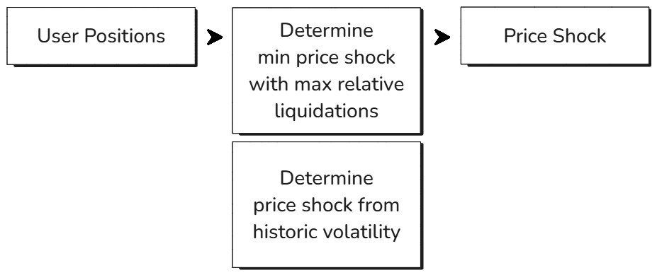
Note: A good approach here can be to calculate the price shock using one method and use another approach to validate the practicality of the derived price shock.

2. Determine the Liquidatable Collateral and Debt

With the chosen price shock we can model and ultimately compute liquidators' profits. For this, we will need the pools where liquidators will eventually make trades. To derive these pools mathematically, we need to know the assets that a liquidator might encounter while liquidating several positions.

In this step, we find the collateral assets that can get liquidated when the derived price shock is applied. Similarly, for those positions, there must be some outstanding debt that must be repaid to get the collateral.

The function that determines these liquidatable positions works with an isolated or siloed market (e.g. crvUSD/LlamaLend) as well as pool-based lending markets where risk is shared across all the assets (e.g. Aave). A key component here is the market logic that determines if a user is liquidatable. This can vary from protocol to protocol and thus this step is market or protocol-dependent. It might even require additional inputs to determine the liquidatable positions.

3. Determine the Global Liquidity

This step is the outcome of the previous step. Here we quote multiple DEX aggregators and develop a mathematical function that is a proxy for the liquidity between a pair of tokens and the slippage relationship between them.

The first substep is to determine the pairs for which we need to develop the liquidity relationship. To determine this we need to look at the liquidator's path. To liquidate this position, a liquidator will execute the process atomically. They will initiate a flashloan (FL_TKN) and repay the liquidatable positions (BORa, BORb, BORn) in exchange for the underlying collateral (COLa, COLb, COLn). The liquidator would make the following actions in their transaction:

1. Borrow FL_TKN as a flashloan

2. Swap FL_TKN → BORa & FL_TKN → BORb

3. Repay BORa & BORb

4. Get COLa & COLb

5. Swap COLa → FL_TKN & COLb → FL_TKN

6. Pay interest on the flashloan in FL_TKN

7. Repay the flashloan in FL_TKN

Pay special attention to steps 2 & 5 here, which require liquid pairings to maximize profitability. For the liquidatable collateral and liquidatable debt we need a set of assets that qualify as flashloan tokens (we use USDC, USDT, DAI, and WETH). With this information, we can have all the required pairs.

We use a modified Gompertz curve to establish a relationship between the available liquidity for this pair. This mathematical function is highly customizable, with adjustable parameters that allow for changes in liquidity conditions based on price movements, and has the capabilities to simulate the effects of trades on the liquidity.

The ultimate goal with this mathematical function is to determine the potential losses that can occur in step 2 and 5 when we are computing the liquidator profit.

4. Adjust the Liquidity per the Price Shock

This is a simpler step where we provide data related to the flashloan assets and the price shock. From these inputs we recompute the constants of the mathematical function discussed in the previous step.

With this adjustment, we ensure that the effect of the price shock is applied to the available liquidity as well.

5. Compute Liquidator Profit for Current Scenario

This step calculates how much profit a liquidator could make in the current market scenario. Here's how it works:

1. For each possible asset that could be used for a flashloan (like USDC, ETH, etc.), it:

   • Calculates how much of that asset would be needed to pay off the liquidatable users' debts (flashloan_start)

   • Calculates how much of that asset the liquidator would receive after selling all the collateral (flashloan_end)

   • Determines the profit by finding the difference between what they get back and what they needed to start (flashloan_end - flashloan_start)

2. The function considers:

   • Current market prices of the flashloan assets or the updated price if the price shock is applied to a flashloan asset.

   • Trading fees and slippage (price impact when making large trades)

   • The need to convert between different assets (e.g., if debt is in USDC but collateral is in ETH)

3. Finally, it identifies which asset would be most profitable to use for the liquidation by comparing all possible scenarios and returns the details of the most profitable option.

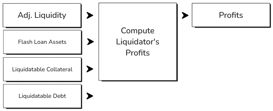
Think of it like a sophisticated calculator that helps us understand the liquidators' possibilities:

• Which asset they should borrow to start the liquidation

• How much they need to borrow

• How much they'll get back

• What their expected profit will be

This step also acts as a validation layer for the current caps and market behavior.

5. Compute Liquidator Profit for the Scaled Scenarios

The next step is to create a hypothetical model of scaled borrower distribution (i.e. maintaining the same health) and to recalculate the profits.

The whole point of scaling is to determine the maximum liquidatable collateral that can be profitably liquidated. The assumption here is that user behavior is kept constant while scaling. This can be examined by scaling the already derived liquidatable collateral and liquidatable debt.

Scaling is nothing but a multiple getting multiplied by the liquidatable collateral and liquidatable debt. With this new liquidatable collateral and liquidatable debt, the profits can increase or decrease depending on the liquidity depth capable of absorbing the liquidation event.

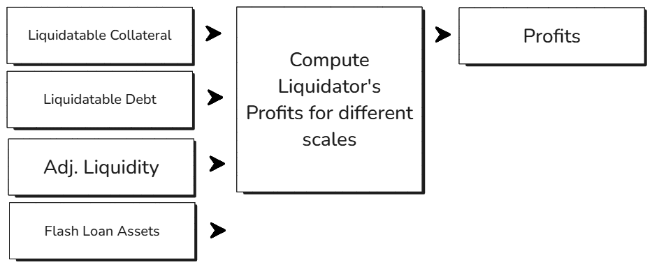
Once we run this process at different scales, here is the trajectory of liquidator profits:

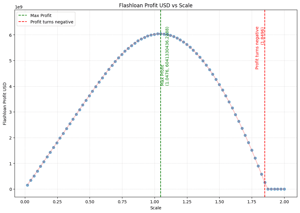
Profits will stay high so long as the price impact is minimal. With the scale value, where profits are maximized, we can be confident in saying that liquidators will profitably liquidate the relevant positions and thus ensure the market remains free from accruing bad debt. This remains true for a hypothetical price shock when the liquidatable collateral is as high as the scaled liquidatable collateral, allowing us to determine if the protocol is overexposed to a given asset or can safely increase its exposure.

6. Translating Scale to a Recommendation

The general idea here is to scale the current supply cap or debt ceiling such that the recommended cap is the current liquidatable collateral * scale. Once this is done we add a condition that caps the magnitude of the increase (a max condition such that the ceiling can only be increased by a fixed proportion in a single epoch). Constraining the recommended cap ensures that transient conditions don't allow for an overcorrection in the recommendation which may be temporarily skewed, for example, by short-term liquidity incentives or borrow actions by whale addresses. It also ensures that we always address the most recent borrower behaviors in each epoch.

It is inherently presumed that the recommendation will reference the market from where the borrower positions are taken. New markets lack data about borrower behaviors. A proxy for determining a reasonable recommendation for a new market without any user behavior is to take user positions from a related asset. For example, if you have a wrapped BTC version of your own (abcBTC) and you want to derive a recommendation, you can use the WBTC market borrower distribution and use the liquidity of abcBTC to determine the liquidator profits.

This analysis of translating the scale value to a recommendation hugely depends on the protocol or market under consideration. Since there are unique properties of each lending platoform, the details of deriving a recommendation for specific protocols will be described in the following section on crvUSD and LlamaLend.

Protocol-Specific Methodology: crvUSD/LlamaLend

This section details the relevant modifications to the general methodology that are required to realistically model the crvUSD mint markets and LlamaLend lending markets. There are two primary considerations:

1. Global Liquidations: There are more significant lending markets on the chains where Curve is active, so we need to take those into consideration.

2. Soft Liquidations: crvUSD uses a novel liquidation mechanism, so we need to model this accurately to assess its capability for absorbing liquidation pressure.

Global Liquidations

When deriving the price shock by computing the liquidatable collateral, we need to consider the liquidations that can happen ecosystem-wide. Since there are other bigger markets than Curve, we need to consider them. Aave is a good example of this. We therefore take into account the potential liquidations on analogous Aave markets for the chosen price shock. These potential liquidations will have an impact on global liquidity (resulting in losses from collateral asset selloff) and would impact the liquidator's profits. In the case of crvUSD and LlamaLend, the analogous Aave market is modeled simultaneously.

Once we have the liquidatable collateral and liquidatable debt quantities for the Curve market and the Aave market (or any other reference market that can pose substantial liquidation volumes during a price shock), we can determine a price shock value. This represents the ecosystem-wide influence that a hypothetical liquidation event could have on our target market.

Soft Liquidations

Computing the liquidatable collateral for a certain price is very straight forward in the case of Aave. We just need the e-mode params, asset params, and price assumption to compute the health, which will allow us to determine the liquidatable collateral and debt. Curve is not so straight forward, as we need to consider its unique "soft liquidation" mechanism. As the collateral price drops, arbitrageurs will swap the borrower's collateral into crvUSD, allowing the user to avoid a painful liquidation event.

There is a caveat that arbitrage will incur a gradual cost, which is variable depending on liquidity conditions, volatility, and arbitrage efficiency. The borrower can become "hard liquidated" (a conventional liquidation) if their position health is substantially eroded from this process. Arbitrageurs need incentives to swap the borrower's collateral to crvUSD and these incentives are taken from the collateral value itself, incurring losses in exchange for preserving the solvency of the position. Hard liquidation can occur somewhere within the bounds of the soft liquidation range, including when the collateral's market price is increasing within that range. This mechanism makes it difficult to compute the liquidatable collateral for a given price point.

Soft Liquidation Efficiency

For the initial iteration, we came up with a concept of soft liquidation efficiency as a parameter. This can be thought of as the collateral value (%) retained after swapping 100% of the collateral inside a price band from collateral asset to crvUSD. As an example, consider a user having a WBTC collateral value equivalent to 10,000 crvUSD and this collateral is spread across 5 bands. When the oracle price of the collateral asset moves across a band, the WBTC in that band is swapped to crvUSD. If the soft liquidation efficiency is set to 95%, the user will have 4*10000/5 = 8000 crvUSD worth of WBTC and (1*10000/5)*95% = 1900 crvUSD left once the price moves across 1 band. Their position will now have the equivalent value of 9,900 crvUSD and will have lost 100 crvUSD in soft liquidation.

With this parameter, we pick a user and try to liquidate the position. The price input for this check is the average price of each band where that user has provided their collateral. There can be multiple price points where a user's health dips below 0. From here, we find the price where the liquidatable collateral (asset other than crvUSD) is at its maximum. After we have done this for all the users, we can get the price vs liquidatable collateral chart. As a reminder, when we say liquidatable collateral we mean the asset token and not the crvUSD token value.

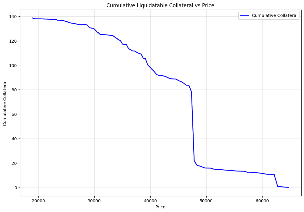
As an example, the chart above shows the cbBTC quantity on the y-axis and the price that can cause the corresponding liquidations on x-axis. The result is the same as simulating a price path (instead of a price point) and determining the liquidations. This approach is faster and more efficient than simulating a dedicated price path where we need to consider a specific path, volatility, and other market conditions. The assumption here is that soft liquidation losses are constant and depend on the collateral value in the bands.

Note: We will be addressing this assumption in a future iteration of this methodology to improve the precision. This is an inherently probabilistic component that can benefit by accounting for observed arbitrage behavior for a particular market.

crvUSD-specific Methodology

With a projected price shock value that accounts for liquidation pressure on significant markets, we can conduct the same steps as discussed in the general methodology to determine a scale value. First, we declare the following:

• Assume the debt ceiling is equal to the variable current_debt_ceiling

• Assume the current collateral is equal to the variable as current_collateral

• Assume the applied price shock is equal to the variable hyp_price

• Assume the total liquidatable for a price shock is hyp_liquidatable_collateral. This is nothing but a sum of hyp_liquidatable_collateral_aave and hyp_liquidatable_collateral_curve

Let's assume the scale comes out as 2. A scale of 2, concludes that for a price shock of hyp_price, 2*hyp_liquidatable_collateral quantity of assets can be profitably swapped to carry out liquidations. We need to frame a scenario where

is the liquidatable collateral for hyp_price price shock.

If we assume the user behavior to be constant on Curve, and if we assume that the borrower behaviors and positions stay constant on Aave, the Curve positions can be scaled such that the liquidatable on Curve after this scaling + liquidatable collateral on Aave is equal to new_hyp_liquidatable_collateral. Let's call this scale_curve. Here this new scale is calculated as

For the current collateral backing the current borrowing, if the liquidatable collateral is to be increased to (new_hyp_liquidatable_collateral - hyp_liquidatable_collateral_aave), the debt should be increased in a way where the final collateral backing it is equal to

This is nothing but

Recommendation Bounds

We advise to have a max_ceiling_multiple and max_floor_multiple while increasing this cap. The purpose of this max_ceiling_multiple is a precaution against the drawbacks of the stacked assumptions. It is better to increase the ceiling multiple times over regular epochs to reach the new_debt_ceiling mark. This way we always consider the latest changes in user positions and user behaviors.

The final recommendation for cases where scale_curve > current_debt_ceiling will therefore be defined as

and for cases where scale_curve < current_debt_ceiling it will be defined as

where 1.5 is the max_ceiling_multiple and 0.8 is the max_floor_multiple.

In future versions of this methodology, we intend to reduce uncertainty from the assumptions and carefully craft the max_ceiling_multiple and max_floor_multiple parameter in accordance with the assumptions.

Note: When we say user positions are constant, it means the position remains the same (there is always someone to fill up a similar position if a position chooses to leave). When we say user behavior is constant, it means the quantities of the collateral and debt can vary but in proportional terms.

Example - cbBTC Debt Ceiling for crvUSD

Curve mint market are bounded by a defined borrow cap and its markets are isolated and one way (can only borrow crvUSD against a collateral asset).

Since Curve is a smaller market compared to markets like Aave, we need to consider the effect of the price shock on the Aave markets, while making a recommendation for the cbBTC market on Curve.

We use WBTC borrower behavior as a proxy for cbBTC. This assumption is reasonable since these are both custodial BTC tokens issued on Ethereum and in direct competition for users.

Using Curve's WBTC borrower distribution, we can model the cumulative liquidatable collateral. The chart below shows the liquidatable collateral vs price.

Since we are considering the Aave markets, we need to check the cumulative liquidatable collateral for Aave. The chart below shows the liquidatable collateral vs price for cbBTC on Aave. We are using the cbBTC market from Aave rather than WBTC because a cbBTC market is already established and would impact the new cbBTC market on Curve.

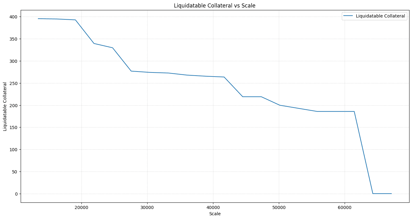
We assume a 10% price shock ($60,000 to be precise, which is reflective of the potential volatility BTC has historically experienced). It turns out that ~200 cbBTC becomes liquidatable when considering both the WBTC market on Curve and the cbBTC market on Aave.

Upon scaling, we get the following chart:

The scale is ~1 (1.0476), meaning if we set the debt ceiling for cbBTC based on the current debt from the WBTC market on Curve (this was ~22m crvUSD at the time of the analysis), liquidators will be profitable for the applied price shock. Note this is also assuming the borrower positions will be the same for cbBTC as for WBTC.

Since we cannot be 100% certain about the alignment of the borrower distribution for cbBTC compared to WBTC, we need to quote something less than the scale we derived (i.e. the conservative approach). Once the market is populated, we can use the actual user behavior to make more calculative and confident quotes for the debt ceiling. We may conclude that a debt ceiling for cbBTC that is slightly below the outstanding debt in the crvUSD WBTC market at the time of analysis is a suitably conservative debt ceiling for market deployment (in this case, around 20m crvUSD).

It is still possible for liquidators to be profitable until a scale of ~1.8x. Given the current scenario where liquidatable WBTC is 180 on Aave and liquidatable cbBTC is 20 on Curve, we can scale the total liquidatable (200 cbBTC) 1.8x and determine an aggressive debt ceiling for crvUSD as follows:

• 200 * 1.8 = 360 (total_liquidatable cbBTC in our hypothetical scenario)

• Liquidatable on Aave = 200 (since we assume nothing is being changed on Aave)

• 360 - 200 = 160 (new_liquidatable on curve)

• 160 / 20 = 8 (new_scale for curve)

• 8 * 22m = 176m (aggressive crvUSD debt ceiling for cbBTC at 1.8x scale)

While the aggressive debt ceiling may still allow liquidations to process, it pushes the limits of liquidity depth and will likely cause a substantial price impact in an adverse scenario. It may also be that a future liquidation event is more extreme than we account for in our model, increasing the risk of bad debt. For these reasons, we base our recommendation on the point of maximum liquidator profits.

In this case, our recommendation for market deployment would be to set the cbBTC debt ceiling at a conservative value of 20m crvUSD and review it after a reasonable period of 1-2 months. Depending on the demand for debt from the market and borrower behavior/liquidity trends, the ceiling could be revised upward, potentially slightly beyond the point of maximum liquidator profits. The advantage of this approach is we can offer the DAO a range of debt ceiling values and inform expectations about the relative risk of applying a debt ceiling at or beyond the point of maximum liquidator profit.