Useful links:

• Curve Market Health Risk Portal

Introduction

This report thoroughly explains the methodology powering our quantitative Market Health Scores, a scoring framework for identifying the health of DeFi lending and stablecoin CDP markets and relative market risk associated with the underlying collateral. An initial implementation of the LlamaRisk Market Health Scores has been done for Curve's crvUSD mint markets, with plans to expand to LlamaLend markets soon.

Market Health Scores are an aggregation of several risk categories, each involving a quantitative evaluation of the target market's dynamics and the properties of the underlying collateral. Ultimately, our goal is to encompass all relevant factors in determining a market's health in a single score that can then be displayed on market UI pages to inform users of risks in the most direct way possible. This document will explain the evaluation process for each health category.

The Market Health Scores Risk Portal may also be a useful tool for protocols looking to integrate with LlamaLend markets and understand their risk. The relevant input data and derived scores for each category should be independently verifiable to ensure comprehensibility and build confidence in the significance of the final score. Therefore, a breakdown of each category and all relevant data is made available for each Market Health Score on a dedicated LlamaRisk Risk Portal page.

Section 1: Foundation of Market Risk Assessment

This section will introduce the guiding principles from which we have devised a comprehensive Market Health Scoring framework. This includes identifying relevant risk signals and evaluating metrics with a process that can be transferable across markets. There is a special consideration in determining what constitutes safe or unsafe market conditions and developing a methodology that reliably evaluates markets that differ in their properties and intended use cases.

1.1 Core Risk Principles

The foundation of our risk assessment methodology centers on two key market participants: lenders and borrowers. Each has distinct risk concerns that must be carefully balanced to ensure market stability. Risk evaluation also encompasses properties of the underlying collateral that inform its risk profile (e.g. liquidity depth and volatility) and behaviors specific to the target market (e.g. borrower distribution and collateralization ratio).

1.1.1 User Protection

Lender Protection

Lenders primarily need the assurance of principal safety. This manifests in two critical ways:

1. Protection against losses through efficient liquidation mechanisms

2. Ability to exit positions when needed (market liquidity)

While interest rate models play a role in managing liquidity risk through utilization curves, our initial methodology focuses on the more fundamental risk of principal protection.

Borrower Protection

Borrowers face a more complex set of risks:

• Liquidation risk from price volatility or oracle inaccuracies

• Rate stability and predictability

• Fair and accurate pricing mechanisms

1.1.2 Key Risk Factors

These participant's needs translate into four fundamental areas that determine market health. Three of these general categories are addressed in the initial implementation of the LlamaRisk Market Health Scores, with the Oracle category being addressed in a future iteration. The three categories we address currently are:

1. Liquidation Efficiency

   • Liquidation mechanisms (and soft liquidation arbitrage in the case of crvUSD) must function smoothly

   • Liquidators and arbitrageurs need proper incentives and the ability to act quickly

2. Asset Characteristics

   • Underlying volatility patterns

   • Price momentum and trends

   • Market depth and liquidity

3. Market Mechanics

   • Collateral ratio distributions

   • Position concentration

   • Liquidation thresholds

The additional category to be addressed in a future iteration include:

1. Price Accuracy

   • Oracle prices must reliably reflect market reality

   • Resistance to manipulation attempts

   • Minimal deviation from true market prices

These factors don't exist in isolation - they interact and amplify each other. A comprehensive scoring system must account for both individual metrics and their interconnected effects on overall market stability.

1.2 Understanding Risk Through Comparative Analysis

The core of our scoring methodology relies on two complementary approaches to measure risk: relative comparisons and benchmark comparisons.

1.2.1 Relative Evaluations

Relative Comparisons (30D vs 7D) reveal important trend changes and emerging risks by comparing recent market behavior against medium-term market behavior. For example, if soft liquidation responsiveness has declined significantly in the past week compared to the monthly average, this could indicate deteriorating market efficiency - even if the absolute values are still within acceptable ranges.

Why Relative Comparisons Matter

Relative comparisons act like an early warning system. When a previously stable market shows a 20% increase in soft liquidations over the past week, that trend matters regardless of whether the absolute number is still "acceptable". These comparisons can reveal:

• Deteriorating market conditions before they breach critical thresholds

• Changes in participant behavior or market dynamics

• Emerging risks that might not yet show up in absolute metrics

1.2.2 Benchmark Evaluations

Benchmark Comparisons provide essential context by measuring against established standards or theoretical limits. While more qualitative in nature, we constrain these benchmarks to quantitative measures where possible. For instance, comparing current collateral ratios against historically proven safe ranges helps identify when markets drift into riskier territory.

Why Benchmark Comparisons Matter

Benchmark comparisons provide crucial context and boundaries. A market might show stable or even improving relative metrics while operating in dangerous territory. For example:

• A collateral ratio that's been steadily low for weeks might look "fine" in relative terms

• An asset's volatility might be consistently high but show no recent changes

• Critical thresholds exist regardless of recent trends

1.2.3 Synergy in the Dual Approach

The real power comes from combining these views:

1. Benchmarks tell us if we're in a safe operating range

2. Relative changes tell us which direction we're heading and how fast

Together, they help distinguish between:

• Temporary fluctuations vs concerning trends

• Normal market behavior vs potential systemic issues

• Minor risks vs critical situations requiring intervention

The power of this methodology comes from combining both perspectives. A market might look healthy when measured against benchmarks, but relative comparisons could reveal concerning trends. Conversely, short-term relative changes might appear alarming until placed in a broader context through benchmark comparison.

This combined approach is particularly important because risks in one area often amplify risks in others. Consider a scenario where:

1. Relative comparison shows increasing asset volatility (7D vs 30D)

2. Benchmark comparison reveals an above-average concentration of positions in soft liquidation

While each factor alone might be manageable, their combination significantly increases the risk of cascading liquidations. Our scoring system accounts for both perspectives when calculating a final category score. The result is a more nuanced and reliable risk assessment that captures both immediate market dynamics and longer-term stability factors.

1.3 Scoring Function Analysis

The implementation of Market Health Scores for each category involves a common scoring logic that is modified by the desired attributes of the observed metric. The score_with_limits function implements a piecewise linear scoring system that converts input values into normalized scores between 0 and 1.

def score_with_limits(score_this: float,
                      upper_limit: float,
                      lower_limit: float,
                      direction: bool,
                      mid_limit: float = None) -> float:
    """
    Score the market based on the collateral ratio 
    comparison

    Args:
        score_this (float): Value to be scored
        upper_limit (float): Upper boundary for scoring
        lower_limit (float): Lower boundary for scoring
        mid_limit (float): Middle point representing 
                           0.5 score
        direction (bool): If True, higher values get 
                          higher scores
                          If False, lower values get 
                          higher scores

    Returns:
        float: Score between 0 and 1
    """

    if mid_limit is None:
        mid_limit = (upper_limit + lower_limit) / 2

    if direction:
        if score_this >= upper_limit:
            return 1.0
        elif score_this <= lower_limit:
            return 0.0
        else:
            # Score between lower and mid
            if score_this <= mid_limit:
                return 0.5 * 
                (score_this - lower_limit) / 
                (mid_limit - lower_limit)
            # Score between mid and upper
            else:
                return 0.5 + 0.5 * 
                (score_this - mid_limit) /
                (upper_limit - mid_limit)
    else:
        if score_this >= upper_limit:
            return 0.0
        elif score_this <= lower_limit:
            return 1.0
        else:
            # Score between lower and mid
            if score_this <= mid_limit:
                return 1.0 - 0.5 * 
                (score_this - lower_limit) /
                (mid_limit - lower_limit)
            # Score between mid and upper
            else:
                return 0.5 - 0.5 * 
                (score_this - mid_limit) /
                (upper_limit - mid_limit)

    # Ensure score is between 0 and 1
    return max(0.0, min(1.0, score))

The function is demonstrated through three different scenarios:

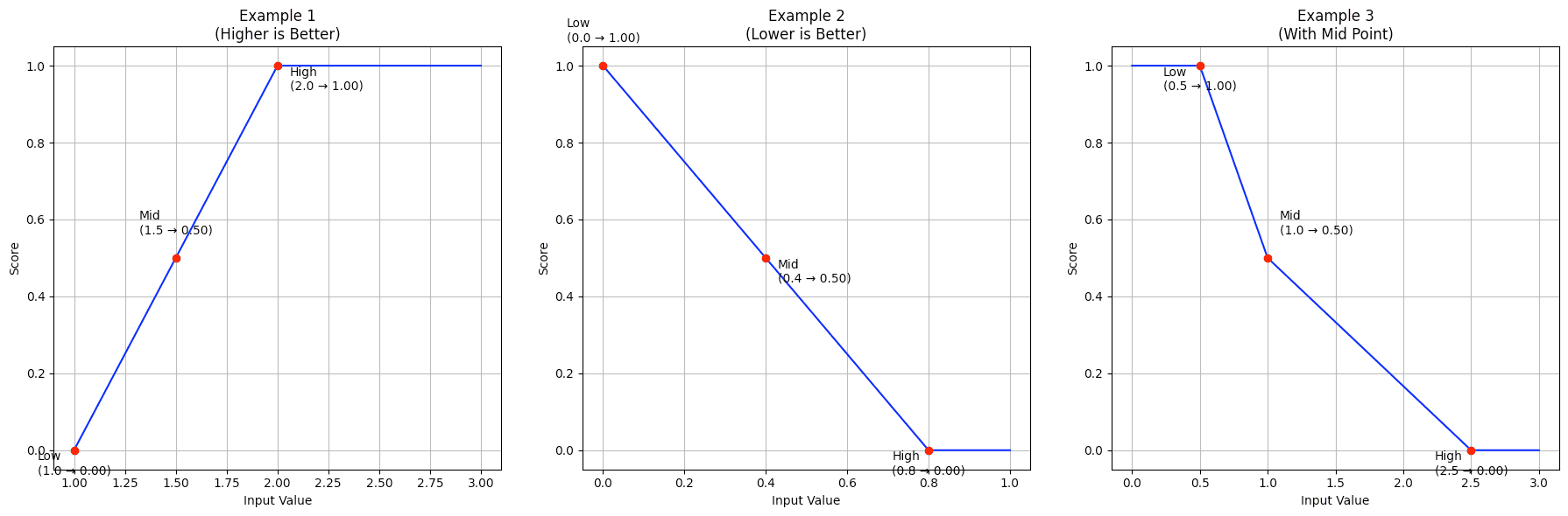
1.3.1 Example 1: Higher is Better

This scenario demonstrates scoring where higher input values are preferred:

• Low (1.0) → Score: 0.00

• Mid (1.5) → Score: 0.50

• High (2.0) → Score: 1.00

• Any value > 2.0 maintains a score of 1.00

score = score_with_limits(
score_this=input_value, # Value to be scored
upper_limit=2.0, # Perfect score threshold
lower_limit=1.0, # Minimum score threshold
direction=True # Higher values are better
)

The function creates a linear progression from the lowest score (0.0) at input 1.0 to the highest score (1.0) at input 2.0, with values above 2.0 maintaining the maximum score.

1.3.2 Example 2: Lower is Better

This scenario shows inverse scoring where lower input values are preferred:

• Low (0.0) → Score: 1.00

• Mid (0.4) → Score: 0.50

• High (0.8) → Score: 0.00

• Any value > 0.8 maintains a score of 0.00

score = score_with_limits(
score_this=input_value, # Value to be scored
upper_limit=0.8, # Critical threshold
lower_limit=0.0, # Perfect score threshold
direction=False # Lower values are better
)

The scoring decreases linearly from a perfect score (1.0) at input 0.0 to a minimum score (0.0) at input 0.8.

1.3.3 Example 3: With Mid Point

This scenario demonstrates scoring with a defined midpoint, creating two different slopes:

• Low (0.5) → Score: 1.00

• Mid (1.0) → Score: 0.50

• High (2.5) → Score: 0.00

score = score_with_limits(
score_this=input_value, # Value to be scored
upper_limit=2.5, # Upper boundary
lower_limit=0.5, # Lower boundary
direction=False, # Lower values are better
mid_limit=1.0 # Reference point for 0.50 score
)

The scoring has different rates of change below and above the midpoint (1.0), allowing for a more nuanced evaluation.

1.3.4 Key Features

1. Linear Interpolation:

   • Smooth, predictable scoring between threshold points

   • Different slopes possible before and after the midpoint

2. Configurable Parameters:

   • Direction: Can handle both "higher is better" and "lower is better" scenarios

   • Thresholds: Customizable upper and lower limits

   • Optional midpoint: Allows for asymmetric scoring ranges

3. Bounded Results:

   • All scores normalized between 0 and 1

   • Clear saturation points at upper and lower thresholds

Section 2: Risk Categories

This section will explain the Market Health categories and the indicators from which the category score is derived. Each category score is weighted to aggregate an overall Market Health Score with respect to the relative significance of the category. Category weightings are given below:

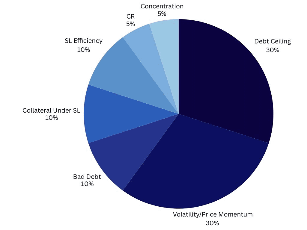
The health categories that make up our overall Market Health Score are given in the table below.

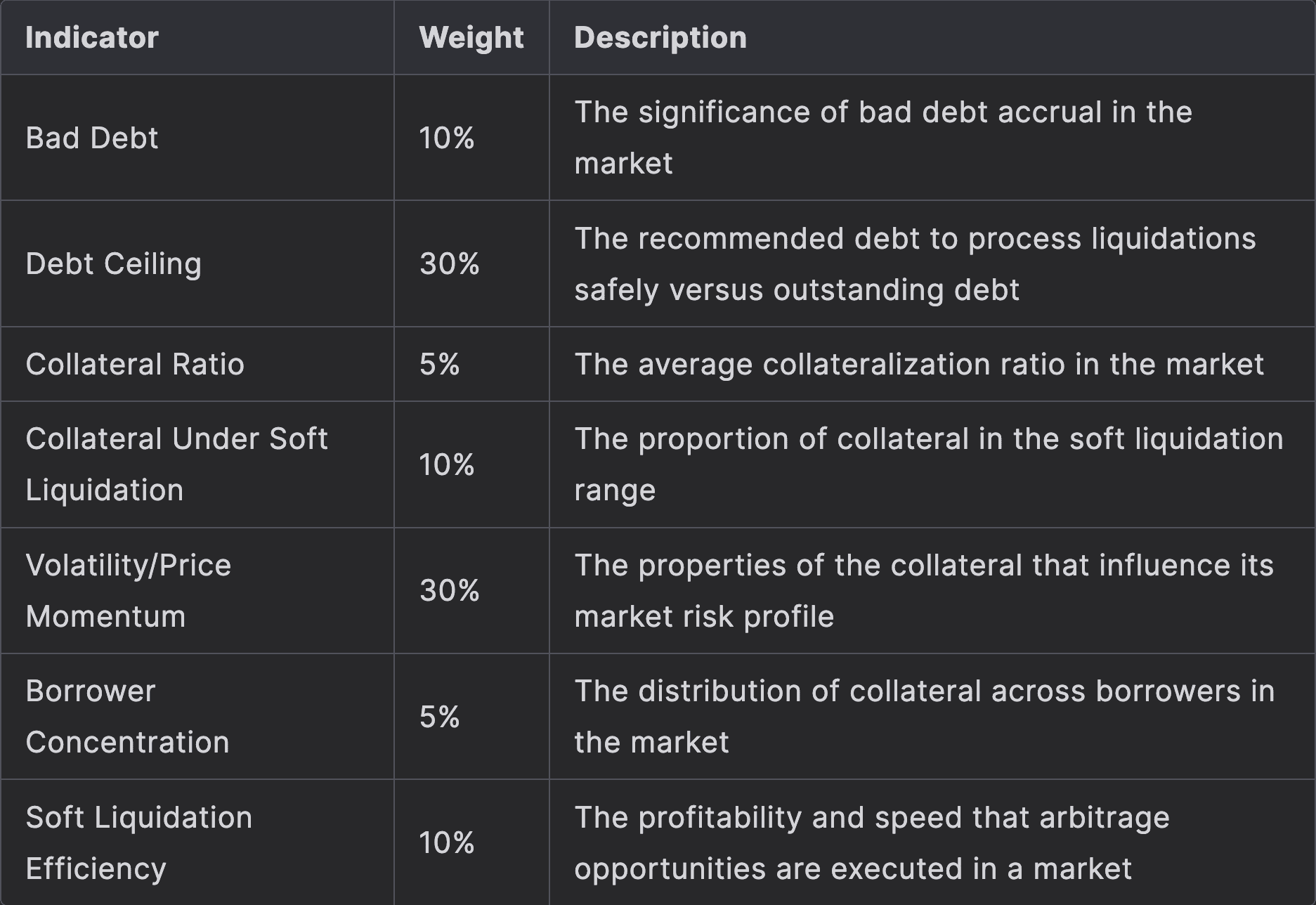
Note that we may revise the scoring framework with additional categories or refine the weighting of each category to align with our assessment of accurately conveying overall market health. Any alterations to the framework can be verified in the LlamaRisk Risk Portal where all current categories, indicators, and weightings are displayed.

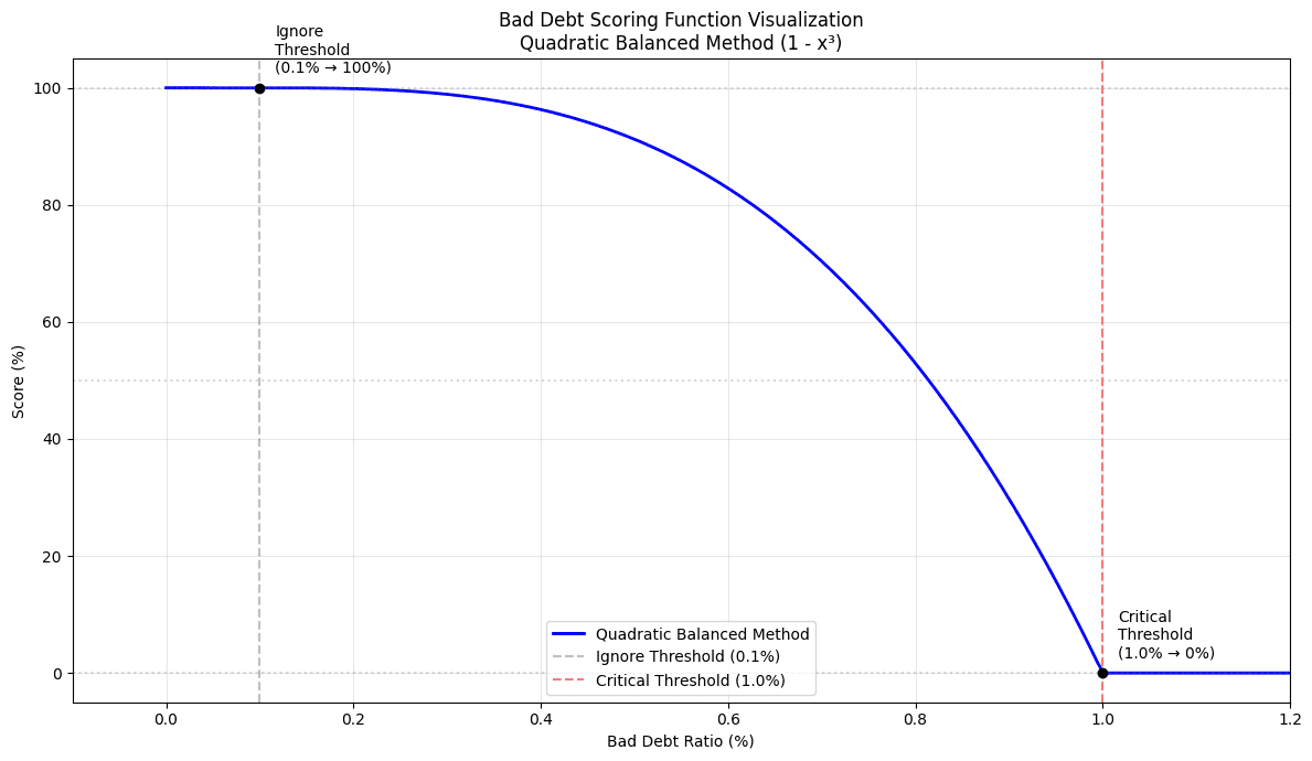
2.1 Bad Debt | Weight 10%

The bad debt scoring system evaluates the health of Curve lending markets by analyzing the ratio of bad debt to total debt. Excessive levels of bad debt in a market may increase the risk of a bank run that may distress the protocol (in the case of CDP stablecoins) or cause illiquidity in the market that prevents lenders from withdrawing and may potentially result in permanent losses for lenders (in the case of lending markets).

The scoring system implements a quadratic model that provides a normalized score between 0 and 1, where 1 represents optimal health (minimal/no bad debt) and 0 represents critical levels of bad debt.

2.1.1 Main Scoring Function

def score_bad_debt(bad_debt: float, 
                   current_debt: float, 
                   method: str = 'quadratic_balanced' 
                   ) -> float:
    """
    Calculates a risk score based on the ratio of 
    bad debt to total current debt.

    Parameters:
        bad_debt (float): Total amount of bad debt 
        in the market
        current_debt (float): Total current debt 
        in the market
        method (str): Interpolation method for 
        scoring curve (default: 'quadratic_balanced')

    Returns:
        float: Score between 0 (high risk) 
        and 1 (low risk)

    Thresholds:
        - Ignore threshold: 0.1% of current debt 
        (score = 1.0)
        - Critical threshold: 1.0% of current debt 
        (score = 0.0)
        - Scores between thresholds use quadratic 
        interpolation
    """

2.1.2 Key Features

1. Threshold-Based Scoring:

   • Ignore Threshold (0.1%): Bad debt below this level receives a perfect score (1.0)

   • Critical Threshold (1.0%): Bad debt above this level receives a minimum score (0.0)

   • Intermediate values are scored using quadratic interpolation

2. Quadratic Interpolation:

   • Uses a balanced quadratic curve for smooth transitions between thresholds

   • Formula: score = 1 - x * x * x where x is the normalized bad debt ratio

   • Provides more nuanced scoring for values between thresholds

3. Visualization Support:

   • Includes plotting function to visualize scoring curves

   • Helps in understanding scoring behavior across different debt ratios

2.1.3 Implementation Details

1. Ratio Calculation:

   bad_debt_ratio = bad_debt / current_debt 
       if current_debt > 0 else 0

2. Threshold Checks:

   if bad_debt_ratio <= IGNORE_THRESHOLD:  # 0.1%
       return 1.0
   if bad_debt_ratio >= CRITICAL_THRESHOLD:  # 1.0%
       return 0.0

3. Score Normalization:

   x = (bad_debt_ratio - IGNORE_THRESHOLD) / 
       (CRITICAL_THRESHOLD - IGNORE_THRESHOLD)

2.2 Debt Ceiling | Weight 30%

The debt ceiling scoring system evaluates the collateral exposure level of Curve lending markets by comparing recommended debt ceilings according to the LlamaRisk Debt Ceiling Methodology against the current debt ceiling and current outstanding debt. The recommended debt ceiling assesses the ability of liquidators to profitably liquidate collateral based on liquidity data, borrower behaviors, and market-wide leverage of the collateral. Outstanding debt that exceeds recommended safe levels may be at higher risk of resulting in missed liquidations and accrual of bad debt in adverse market scenarios.

The scoring system implements a linear scoring model that provides a normalized score between 0 and 1, where 1 represents a safe debt ceiling and 0 represents significant overcapacity.

2.2.1 Main Scoring Function

def score_debt_ceiling(recommended_debt_ceiling: float, 
                       current_debt_ceiling: float, 
                       current_debt: float) -> float:
    """
    Calculates a risk score based on the ratio of 
    recommended ceiling to current ceiling.

    Parameters:
        recommended_debt_ceiling (float): 
        Recommended maximum debt ceiling
        current_debt_ceiling (float): Current total 
        debt ceiling (total_debt + borrowable)
        current_debt (float): Current total debt 
        in the market

    Returns:
        float: Score between 0 (high risk) and 1 
        (low risk)

    Scoring Logic:
        - If current ceiling <= recommended: 
        Perfect score (1.0)
        - If current debt <= recommended: 
        Score between 0.5 and 1.0
        - If current debt > recommended: 
        Minimum score (0.0)
    """

Note that this methodology is specific to the properties of crvUSD mint markets, which impose a max debt ceiling on each CDP market. LlamaLend markets, for instance, do not impose a debt ceiling and therefore require a modified logic based on the market supply and outstanding debt.

2.2.2 Key Features

1. Tiered Scoring System:

   • Perfect Score (1.0): Current ceiling at or below recommendations

   • Partial Score (0.5-1.0): Current debt below recommendations and current ceiling above recommendations

   • Zero Score (0.0): Current debt exceeds recommendations

2. Linear Interpolation:

   • Uses linear scaling between 0.5 and 1.0 for partial scores

   • Formula: score = 0.5 + 0.5 * ((recommended - current_debt) / recommended)

   • Provides proportional scoring for acceptable debt levels

2.2.3 Implementation Details

1. Basic Threshold Check:

   if current_debt_ceiling <= recommended_debt_ceiling:
       return 1.0

2. Debt Level Assessment:

   elif current_debt <= recommended_debt_ceiling:
       return 0.5 + 0.5 * 
              ((recommended_debt_ceiling - current_debt) /
              recommended_debt_ceiling)

3. Critical Level Check:

   else:
       return 0.0

2.3 Collateral Ratio | Weight 5%

The Collateral Ratio scoring system evaluates market health by analyzing both current collateralization levels and their stability over time. Lower collateralization levels in a market are indicative of either aggressive borrower behaviors or distressed market conditions. We consider markets safer when average collateral ratios are stable and do not pose a significant risk to the market's solvency in adverse market scenarios.

The scoring system combines relative (temporal) and absolute (threshold-based) metrics to provide a comprehensive risk assessment of the market's collateralization properties.

2.3.1 Main Scoring Function

def score_with_limits(score_this: float, 
                      upper_limit: float, 
                      lower_limit: float, 
                      direction: bool = True, 
                      mid_limit: float = None) -> float:
    """
    Calculates a normalized score based on value position 
    within defined limits.

    Parameters:
        score_this (float): Value to score
        upper_limit (float): Upper boundary for scoring
        lower_limit (float): Lower boundary for scoring
        direction (bool): True if higher values are better, 
        False if lower are better
        mid_limit (float): Middle point representing 0.5 score 
        (optional)

    Returns:
        float: Score between 0 (high risk) and 1 (low risk)
    """

2.3.2 Key Features

1. Dual Scoring Components:

   • Relative Score (40%): Evaluates CR stability using 7d/30d ratio to assess the trajectory of market CR

   • Absolute Score (60%): Compares current CR against LTV limits considered safe based on the target market's parameters

   • Final Score: Weighted average of both components

2. LTV Range Analysis:

   • Min LTV (Conservative bound): Found from the market's A parameter and the highest possible bands a user could put their collateral into (e.g. 69.0%)

   • Max LTV (Risk bound): Found from the market's A parameter and the lowest possible bands a user could put their collateral into (e.g. 92.0%)

   • Safety Margin: 25% buffer on bounds

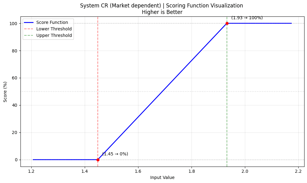
   • Corresponding CR Ranges: For this example, the range is 144.9% - 108.7%. The bounds after applying the safety margin are 193.2% - 144.9%.

3. Scoring Thresholds:

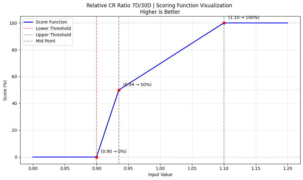
   • Relative: 0.9 (lower) to 1.1 (upper) and midpoint at 0.935 (50% score) for 7d/30d ratio. The midpoint is chosen in a way that if 7d/30d is not changing the score would fall to ~70%

   • Absolute: Based on LTV-derived CR limits with a safety margin

   • Linear interpolation between thresholds

2.3.3 Implementation Details

1. Relative CR Scoring:

relative_cr_score = score_with_limits(
    cr_7d_30d_ratio,  # Current 7d/30d CR ratio
    1.1,              # Upper threshold (110%)
    0.9,              # Lower threshold (90%)
    True,             # Higher values preferred
    0.935
)

2. Absolute CR Scoring:

absolute_cr_score = score_with_limits(
    current_cr,
    1/(0.75 * min_ltv),  # Upper CR threshold with margin
    1/(0.75 * max_ltv),  # Lower CR threshold with margin
    True                 # Higher values preferred
)

3. Final Score Calculation:

final_score = 0.4 * relative_cr_score + 0.6 * 
              absolute_cr_score

2.3.4 Market Examples

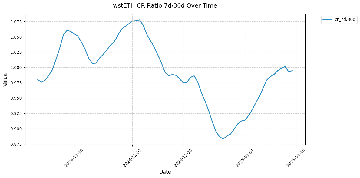
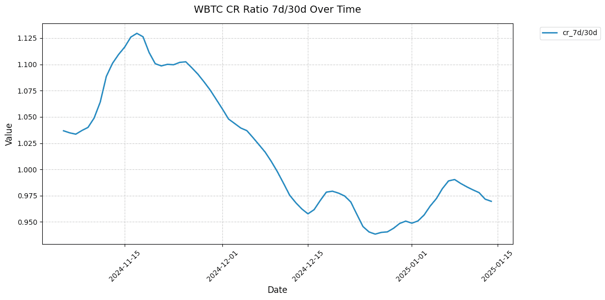
Shown below are 7d/30d collateralization ratios for select markets. This relative metric shows the directionality of the market CR over time normalized to 1.

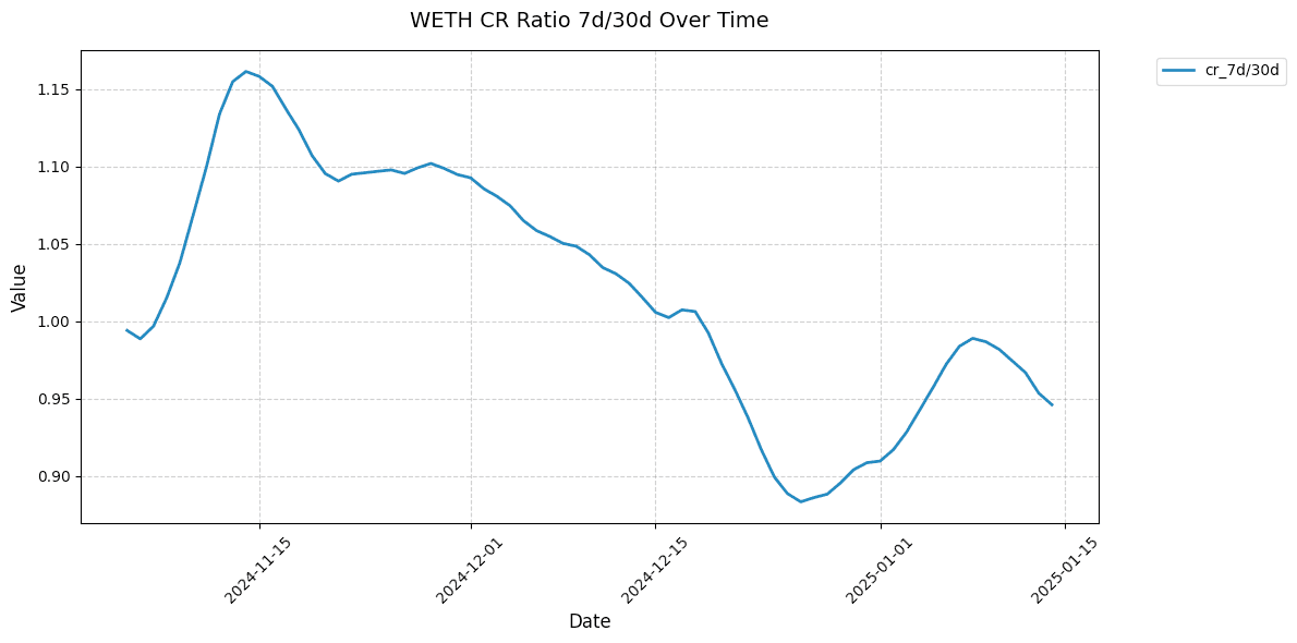
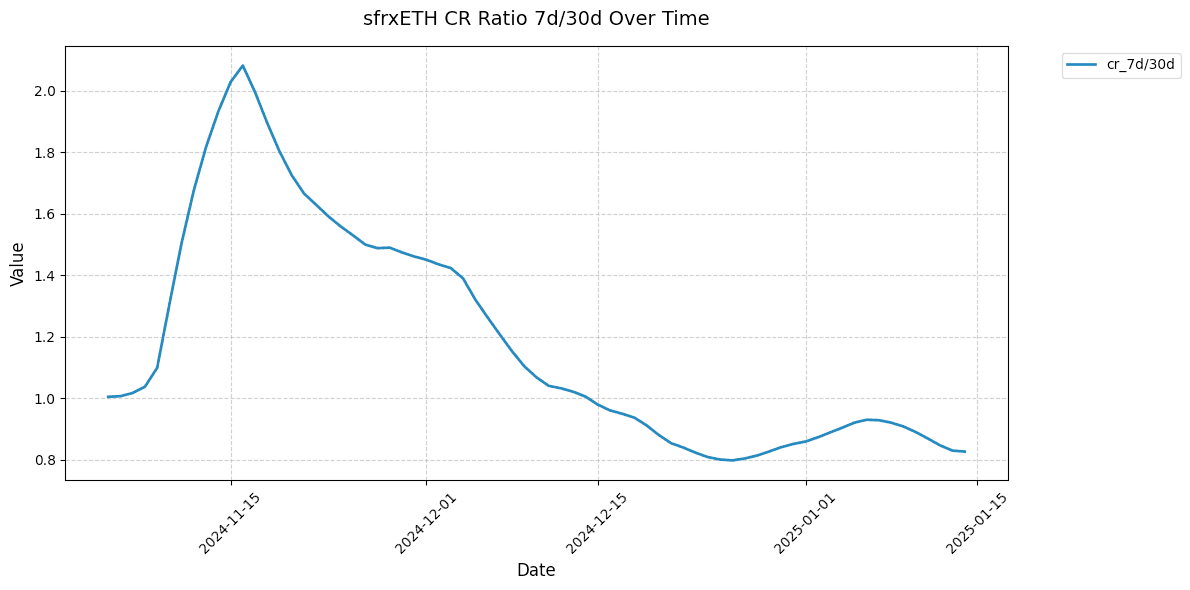
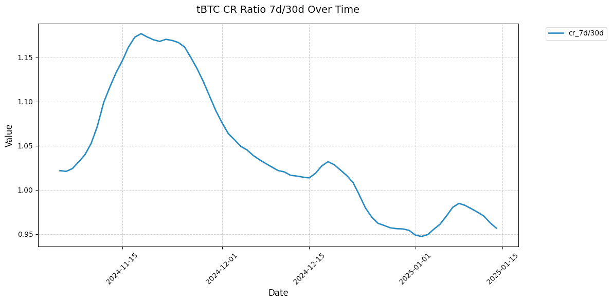
2.4 Collateral Under Soft Liquidation | Weight 10%

crvUSD involves a novel liquidation mechanism whereby soft liquidation precedes and mitigates the risk of hard (irreversible) liquidation. The proportion of collateral in a market that is under soft liquidation will give us foresight as to how much collateral is at risk. A large or increasing portion of overall collateral in soft liquidation indicates adverse market conditions that may threaten the solvency of the market.

This scoring system considers the sum of collateral for all users under soft liquidation / total collateral. It uses the same function as the Collateral Ratio metric and has a similar scoring logic (relative comparison and absolute comparison). The dual evaluation offers a comprehensive assessment of the soft liquidation risk by considering the absolute proportion of collateral under liquidation and the trajectory of that proportion.

2.3.1 Main Scoring Function

def score_with_limits(score_this: float, 
                      upper_limit: float, 
                      lower_limit: float, 
                      direction: bool = True, 
                      mid_limit: float = None) -> float:
    """
    Calculates a normalized score based on value position 
    within defined limits.

    Parameters:
        score_this (float): Value to score
        upper_limit (float): Upper boundary for scoring
        lower_limit (float): Lower boundary for scoring
        direction (bool): True if higher values are better, 
        False if lower are better
        mid_limit (float): Middle point representing 0.5 score 
        (optional)

    Returns:
        float: Score between 0 (high risk) and 1 (low risk)
    """

2.4.2 Key Components

1. Dual Scoring Components:

   • Relative Score: Compares 7-day vs 30-day average of collateral under soft liquidation with a ratio of 7D/30D

   • Absolute Score: Evaluates the current percentage of collateral under soft liquidation

   • Final Score: Weighted average of both components

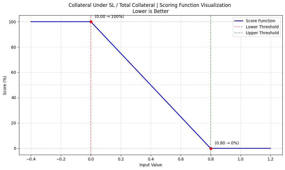
2. Absolute Collateral under SL Analysis:

   • Score is 1.0 if no collateral is under soft liquidation

   • Score is 0.0 if 80% or more collateral is under soft liquidation

   • Linear interpolation between thresholds

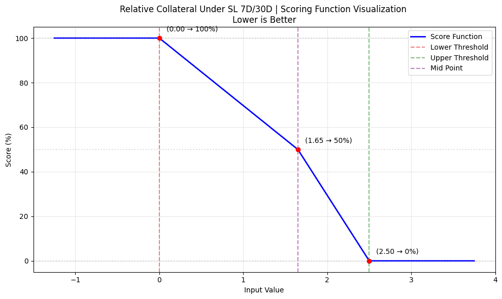
3. Relative Collateral under SL Analysis:

   • Compares 7-day vs 30-day average of collateral under soft liquidation with a ratio of 7D/30D to help identify worsening trends

   • Score is 1.0 if 7D average is 50% lower than 30D average

   • Score is 0.5 if 7D is ~1.65x of 30D

   • Score is 0.7 if 7D matches 30D (ratio = 1.0). This is achieved by adjusting the midpoint to 1.65.

   • Score is 0.0 if 7D is 2.5x higher than 30D

2.4.3 Implementation Details

1. Absolute Score (60%):

abs_score = score_with_limits(
    collateral_under_sl,  # Current collateral under SL
    0.8,                 # Upper threshold (80%)
    0.0,                 # Lower threshold (0%)
    False                # Lower values preferred     
)

2. Relative Score (40%):

rel_score = score_with_limits(
    ratio_7d_30d,  # 7d/30d ratio
    2.5,           # Upper threshold (250%)
    0.5,           # Lower threshold (50%)
    False,         # Lower values preferred
    1.65            # Midpoint (100%)
)

3. Final Score Calculation:

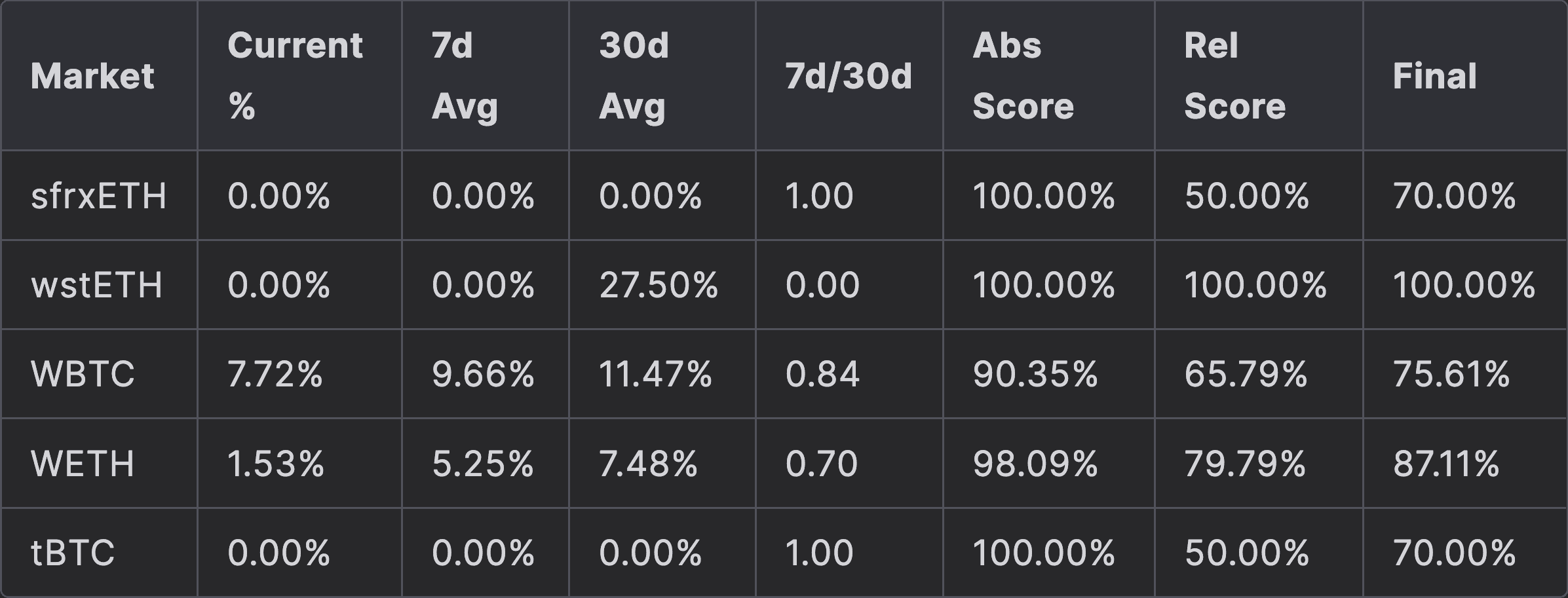
2.4.4 Market Example

A sample analysis from March 2024 is given in the table below to demonstrate the absolute and relative proportion of collateral under soft liquidation, and the implications for the overall score at that point in time.

2.5 Asset Price Momentum & Volatility | Weight 30%

The Volatility Exposure scoring system evaluates market risk through three components: relative volatility changes, Bitcoin correlation, and a Value at Risk (VaR) model. These factors assess market maturity of the underlying collateral to determine the relative risk posed by the collateral. Assets that are immature or excessively volatile may be at greater risk of liquidation and potential market insolvency.

Our scoring system uses the Garman-Klass volatility estimator and provides a normalized score between 0 and 1, where 1 represents stable risk characteristics and 0 represents concerning exposure.

2.5.1 Volatility Calculation

The system uses a modified Garman-Klass volatility estimator that leverages OHLC (Open-High-Low-Close) data for more efficient volatility estimates:

2.5.2 Key Components

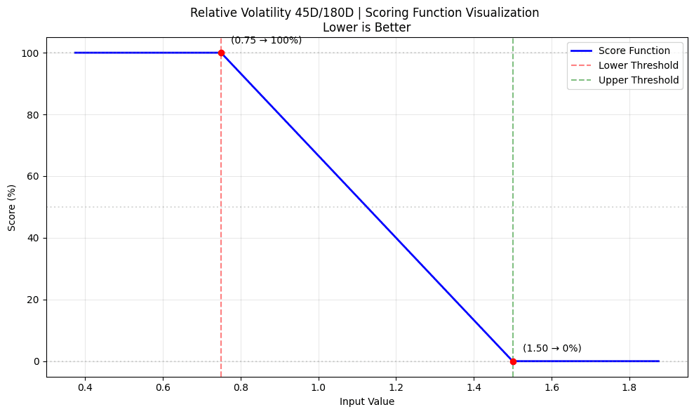
1. Volatility Ratio Scoring | Relative Comparison:

• Compares 45-day vs 180-day volatility windows

• formula: vol_ratio = vol_45d/vol_180d

vol_ratio_score = score_with_limits(vol_ratio, 
                                  1.5, 
                                  0.75, 
                                  False
                                  )

• Score is 0 if recent volatility (45d) exceeds 1.5x the historical volatility (180d)

• Score is 1 if ratio is below 0.75x

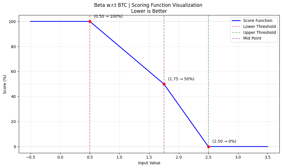
2. Beta Scoring | Benchmark Comparison:

• Measures correlation with BTC price movements, scoring the asset relative to the volatility profile of BTC

• Beta calculation:

beta = correlation * (asset_vol / btc_vol)

• Both asset_vol and btc_vol use the Garman-Klass method

• Beta scoring:

  beta_score = score_with_limits(beta, 
                               2.5, 
                               0.5, 
                               False, 
                               1.75
                              )

• Score is 1 at beta = 0.5

• Score is 0.8 at beta = 1 i.e. BTC derivatives

• Score is 0 if beta exceeds 2.5

3. VaR Scoring | Loss Quantification:

• Uses a Value at Risk model to quantify downside risk based on daily returns.

• The daily percentage change in closing prices is computed first to see how much the price shifts from day to day and then removes any missing values. Next, it identifies the value at the 1st percentile, which represents one of the worst daily losses you might expect. Finally, it converts this loss estimate into a score using set limits, helping to gauge the level of risk associated with such extreme declines.

• VaR scoring:

  var_score = score_with_limits(var_99, 
                               -0.01, 
                               -0.12, 
                               True, 
                               -0.085
                               )

  

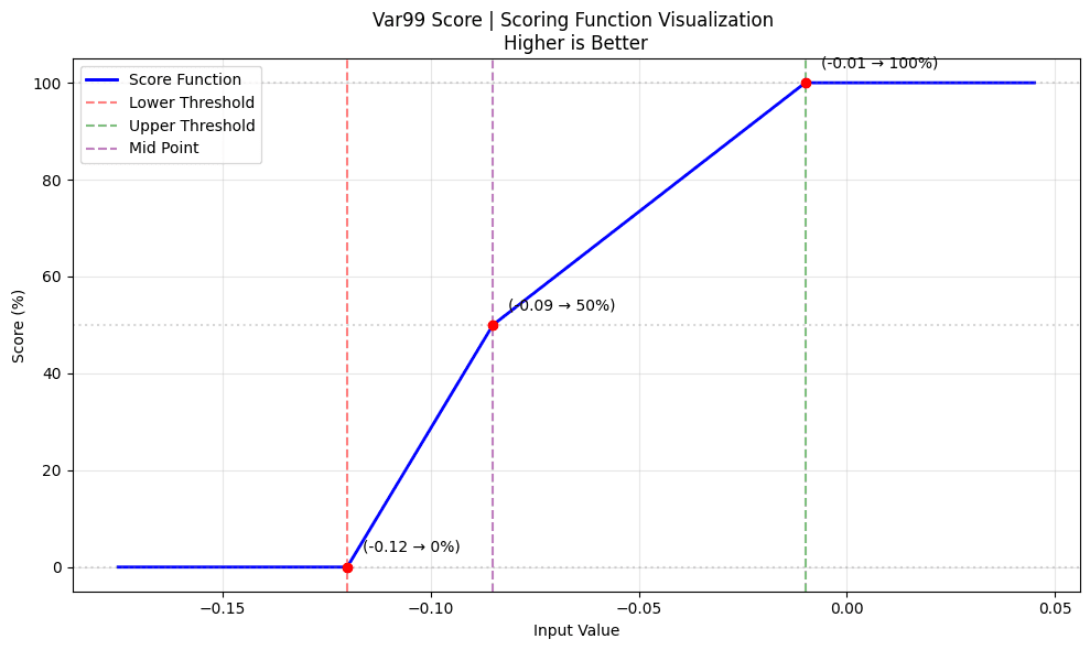
• Interpretation:

  • The VaR score evaluates the risk of extreme daily losses.

  • The scoring function maps the VaR value to a normalized score between 0 and 1 based on predefined limits, where a value closer to the target (here, -0.085) yields a better score.

4. Final Score Calculation:

• The aggregate asset score now combines all three risk measures:

  aggregate_asset_score = (0.3 * vol_ratio_score + 
                           0.3 * beta_score + 
                           0.4 * var_99_score)

• Weighting:

  • Volatility Ratio contributes 30%.

  • Beta Score contributes 30%.

  • VaR Score contributes 40%.

2.5.3 Example Market

This scoring approach combines both temporal volatility changes, BTC correlation, and downside risk (via the VaR model) to provide a comprehensive risk assessment. The Garman-Klass estimator offers more accurate volatility measurements by incorporating high-low ranges, while the beta component and VaR model help assess systematic market risk and extreme loss probabilities, respectively.

A scoring example for WBTC is given below:

2.6 Borrower Concentration | Weight 5%

The Borrower Concentration scoring system evaluates the distribution of debt across borrowers using the Herfindahl-Hirschman Index (HHI). High concentration of debt among a few borrowers indicates general market immaturity and can pose systemic risks to the lending market, as the default of a major borrower could significantly impact the protocol's stability.

The scoring system provides a normalized score between 0 and 1, where 1 represents well-distributed borrowing and 0 represents concerning concentration levels. It combines both temporal changes in the borrower concentration and a comparison against an ideal distribution. The HHI provides a standardized way to measure concentration, while the dual scoring components help identify sudden changes alongside sustained concentration issues.

2.6.1 Main Scoring Function

The HHI, originally developed for measuring market concentration in industries, is particularly suitable for assessing borrower distribution because it:

• Gives more weight to larger debt positions by squaring individual shares

• Has a known minimum value when debt is perfectly distributed

• Increases non-linearly as concentration increases

• Provides a single metric that can be tracked over time

HHI Calculation

The system uses the Herfindahl-Hirschman Index to measure market concentration:

For example, if a market has $10M in total debt:

Scenario 1: Equal Distribution (10 users with $1M each)

HHI = (1M)² + (1M)² + ... + (1M)² (10 times)
    = 10 * (1M)²
    = 10 * (1e6)²
    = 1e13

HHI_ideal = (10M)² / 10
         = (1e7)² / 10
         = 1e13

HHI_ratio = 1e13 / 1e13 = 1.0  # Perfect distribution

Scenario 2: Concentrated (1 user with $9M, 9 users with $100K each)

HHI = (9M)² + (0.1M)² + ... + (0.1M)² (9 times)
    = 81e12 + 9 * (0.1e6)²
    = 81e12 + 9 * 1e10
    = 81.09e12

HHI_ideal = (10M)² / 10
         = (1e7)² / 10
         = 1e13

HHI_ratio = 81.09e12 / 1e13 = 8.109  # High concentration

In Scenario 2, the HHI ratio is almost 8.109x the ideal value, indicating significant concentration risk.

For scoring purposes, it follows the function below:

def score_with_limits(score_this: float, 
                      upper_limit: float, 
                      lower_limit: float, 
                      direction: bool = True, 
                      mid_limit: float = None) -> float:
    """
    Calculates a normalized score based on value position 
    within defined limits.

    Parameters:
        score_this (float): Value to score
        upper_limit (float): Upper boundary for scoring
        lower_limit (float): Lower boundary for scoring
        direction (bool): True if higher values are better, 
        False if lower are better
        mid_limit (float): Middle point representing 0.5 score 
        (optional)

    Returns:
        float: Score between 0 (high risk) and 1 (low risk)
    """

2.6.2 Key Components

1. Dual Scoring Approach:

   • Stability trend monitoring (relative score) assesses changes in market maturity by tracking the directionality of borrower distirbution.

   • Target distribution monitoring (absolute score) assesses the absolute distribution with scores assigned based on an ideal threshold.

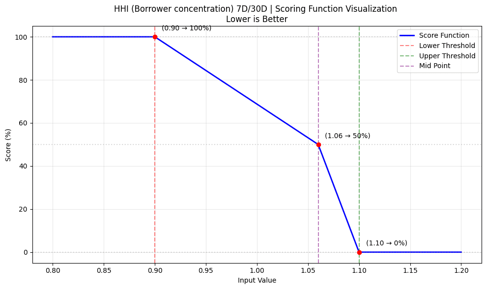
2. Relative Distribution Scoring (50%):

   • Compares recent (7D) vs historical (30D) concentration trends to help identify sudden changes in borrower distribution

   • 1.0 score: 7D borrower distribution is more distributed than 30D distribution

   • 0.7 score: 7D borrower distribution is similarly distributed compared to 30D distribution

   • 0.01 - 0.49 score: Linear interpolation between 110% to 106% deviation in borrower concentration

   • 0.5 - 0.99 score: Linear interpolation between 90% to 106% deviation in borrower concentration

   • 0.0: 7D borrower concentration >10% higher than 30D concentration.

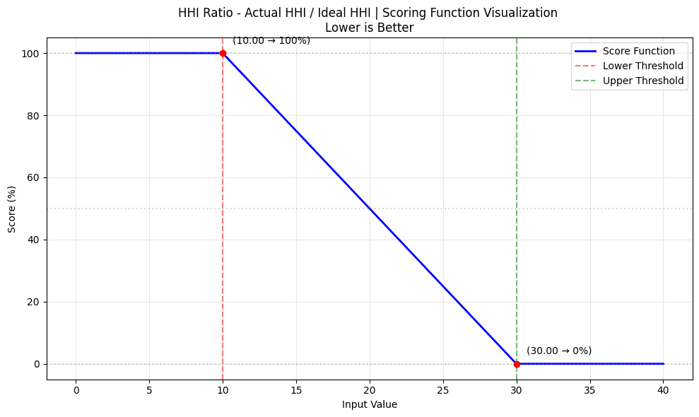
3. Absolute Distribution Scoring (50%):

   • Compares current HHI ratio against ideal thresholds

   • Measures how far current distribution deviates from perfect equality

   • 1.0: Distribution close to ideal (HHI ratio ≤ 10x)

   • 0.5: Moderate concentration (HHI ratio = 20x)

   • 0.0: High concentration (HHI ratio ≥ 30x)

2.6.3 Implementation Details

1. Relative Distribution Scoring (50%):

hhi_7d_30d_ratio = hhi_7d / hhi_30d
relative_borrower_distribution_score = score_with_limits(
    hhi_7d_30d_ratio,  # Recent/Historical HHI ratio
    1.1,               # Upper threshold (110%)
    0.9,               # Lower threshold (90%)
    False,             # Higher values preferred
    1.06
)

2. Absolute Distribution Scoring (50%):

benchmark_borrower_distribution_score = score_with_limits(
    last_row["hhi_ratio"],  # Current HHI ratio
    30,                     # Upper threshold (10x ideal)
    10,                     # Lower threshold (30x ideal)
    False                   # Higher values preferred
)

2.6.4 Market Example

A sample analysis of the crvUSD WETH mint market is given below to demonstrate borrower concentration and the implications for the overall score.

2.7 Soft Liquidation Efficiency | Weight 10%

Soft liquidation efficiency monitors the speed with which arbitrageurs execute trades and the profitability of those trades after an opportunity arises. An active arbitrage market is essential to the design of crvUSD's liquidation mechanism, as it requires efficient arbitrage to preserve borrower position health while in soft liquidation. Inefficient arbitrage can be a sign of immature markets, excessive volatility, or prohibitive gas costs that increase the risk that borrowers can be hard liquidated. This may threaten the solvency of the market in adverse market scenarios.

The scoring system approximates the efficiency of arbitrage events by comparing the deviation between a market's spot price to the oracle price. The distribution of recent historical events are used to assess performance by measuring deviation consistency and most common deviation. This dual scoring method allows for a comprehensive assessment of the market's arbitrage efficiency.

2.7.1 Main Scoring Function

Estimating the exact gains from soft liquidation and classifying arbitrageurs (who seek to profit from soft liquidations) from DEX aggregators is a complex task. We approximate the opportunity for arbitrageurs by using the price deviation of the market's internal AMM price from the oracle price. This price deviation, coupled with the swappable collateral, can be a good proxy to determine the arb opportunity.

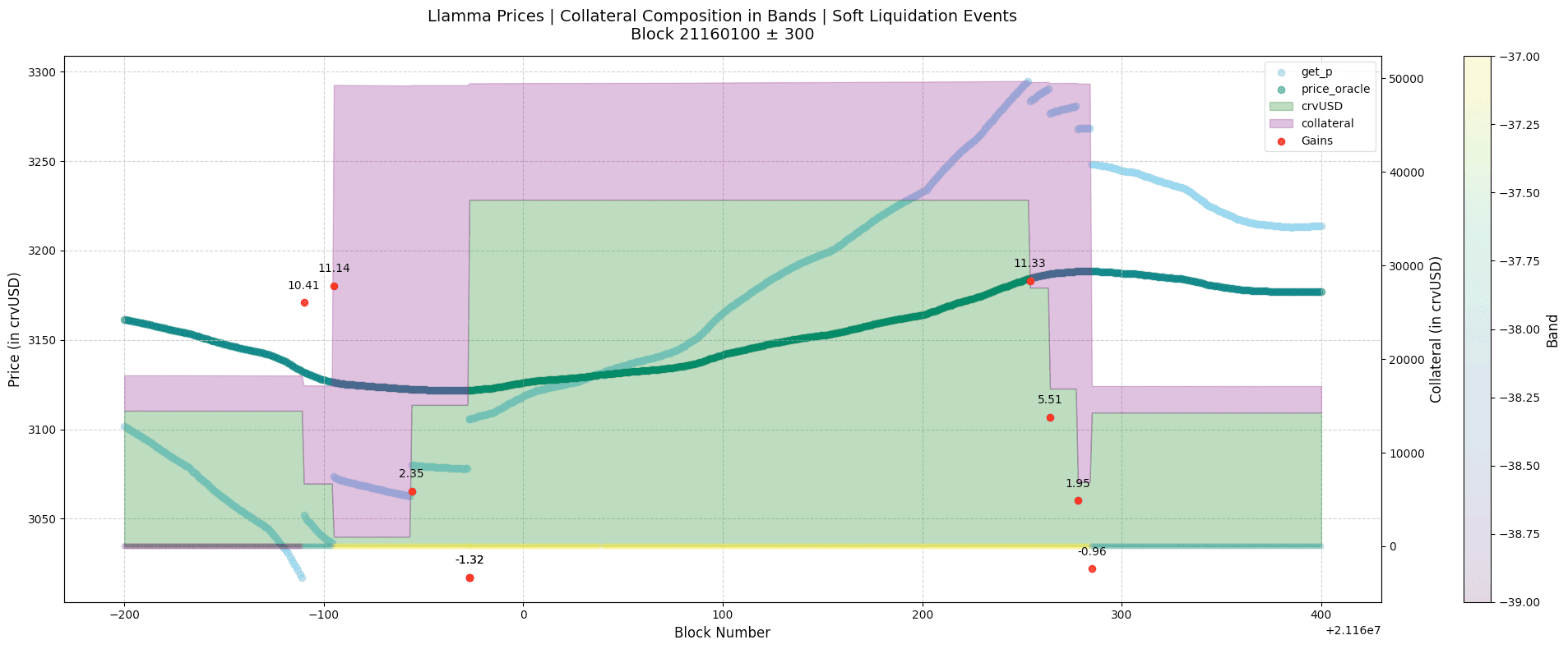
The red scatter in the above chart shows the swap events. The chart shows the oracle price (price_oracle) and the AMM price (get_p). It also shows the active band and the composition through time.

The price deviation is the difference between the oracle price and the AMM price. This deviation is multiplied by the swappable collateral value denominated in crvUSD. This product is used as a proxy for the arbitrage opportunity.

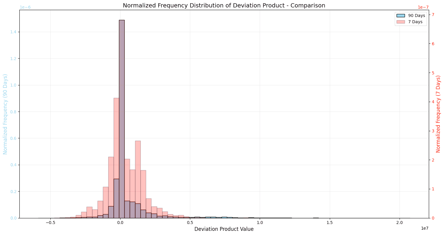
Using this product for n blocks, we construct a distribution of the arbitrage opportunity. This distribution is compared against a relatively larger time window distribution. The distribution peak is near 0 in ideal conditions; the closer the distribution is to 0, the better the market is performing in terms of fulfilling soft liquidations.

2.7.2 Key Components

The arbitrage efficiency is evaluated on two fronts:

1. Distribution spread comparison: how tightly clustered price deviations are, a tighter spread means required arbitrage is happening which is not allowing the price to deviate more.

2. Distribution peak comparison: how close the distribution peak is to 0, considered a perfect efficiency

For both the comparisons, we need some kind of reference or benchmark and we use the larger time frame market performance as a reference. Here is a sample comparison of 90D vs 7D distribution:

A dual scoring approach helps identify different types of inefficiencies:

• High spread score + Low peak score indicates consistent performance but overall poor execution

• Low spread score + High peak score indicates overall good arbitrage performance with relatively high inconsistency

• Low scores in both indicate a generally inefficient market

• High scores in both indicate optimal soft liquidation efficiency

The scoring system rewards:

1. Tight clustering of deviation * swappable collateral (spread score)

2. Deviation * swappable collateral centered near zero (peak score)

3. Consistency with historical patterns (reference comparison)

A high score indicates efficient soft liquidation mechanics where arbitrage opportunities are quickly taken, price deviations are minimal, and market behavior is stable and predictable.

2.7.3 Scoring Components

1. Distribution Spread Analysis (50%):

• Measures how tightly clustered the arbitrage opportunities are

• Uses three statistical measures:

  spread_metrics = {
      'std': Standard deviation of opportunities
      'iqr': Interquartile range
      'range': Total range (max - min)
  }

• Each metric provides different insights:

  • StdDev: Overall variability of opportunities

  • IQR: Spread of middle 50% of opportunities

  • Range: Maximum spread of opportunities

• Scoring formula:

  def spread_ratio_score(test_val, ref_val):
      ratio = test_val / ref_val
      if ratio <= 1:  
          # Tighter spread than reference (good)
          return 50 + (50 * (1 - ratio))  # Score: 50-100
      else:  
          # Wider spread than reference (bad)
          return max(0, 50 * (25 - ratio) / 24)  # Score: 0-50

• Example:

      {
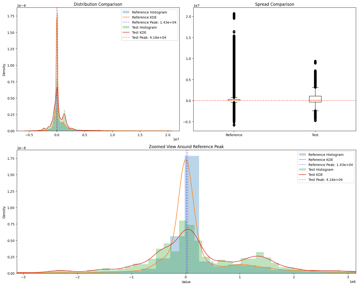
         "spread_analysis": {
             "score": 59.20728624528061,
             "metrics": {
                 "reference": {
                     "std": 1566172.9802697,
                     "iqr": 310276.0281798712,
                     "range": 26639162.349364825
                 },
                 "test": {
                     "std": 1204641.9387078695,
                     "iqr": 1392111.235248369,
                     "range": 14201909.156186275
                 }
             }
         },
         "peak_analysis": {
             "score": 91.62780944807079,
             "metrics": {
                 "reference_peak": 14251.986662063748,
                 "test_peak": 41639.76751948707,
                 "difference_in_std_units": 0.01748707275789,
                 "reference_std": 1566172.9802697,
                 "absolute_difference": 27387.78085742332
             }
         },
         "overall_score": 75.4175478466757
      }

  Following is a visual version of the score derivation where the analysis is run on an example market and two time frames were compared. It corresponds with the example above.

  

2. Peak Location Analysis (50%):

• Measures how close the distribution peak is to zero

• Uses Gaussian KDE to find distribution peaks

• Scoring process:

  1. Find peak of reference distribution

  2. Find peak of test distribution

  3. Calculate difference in standard deviation units

  4. Apply exponential decay scoring

• Scoring formula:

  peak_diff_in_stds = |test_peak - ref_peak| / ref_std
  peak_score = 100 * exp(-peak_diff_in_stds * 5)

• Example:

1. Final Score Calculation:

   overall_score = (spread_score + peak_score) / 2